SMall Is Beautiful v 0.36
philippe.billet@noos.fr
1 Introduction
smib stands for SMall Is Beautiful (a small borrowing to the economist Ernst Friedrich Schumacher) and is a Computer Algebra System (CAS) for Linux. smib is less efficient than other CAS but it is smaller; in fact I wanted to make an educational sofware (smib may be useful in high school or university mathematics), easy to program, easy to understand.
Historically, smib derives from George Weigt’s Eigenmath. Constitutionally, it is a subtle mixture of C++ (or rather C+), of FORTH (for stack) and LISP (for lists). Philosophically, it is an experimental tool in mathematics computer-assisted.
Some fields of application that smib touches:
-
number theory (integer, primality, arithmetic functions, Dirichlet convolution),
-
algebra (polynomial, matrix, rational function, tensor),
-
analysis (trigonometry, special functions, differential calculus, integration, Fourier transform, Taylor sum),
-
differential geometry (curves, surfaces, tensorial calculus),
-
numerical analysis (interpolation, numerical integration, ordinary differential equation, sample manipulation, numerical Fourier transform, differintegration, complex analysis),
-
probality & statistic (expected value, variance, standard deviation, skewness, kurtosis, least square fitting, quantile, stochastic differential equation).
smib naturally supports tensorial structures, and has a pretty good array management. This facilitates the handling of object of type
(xi, f(xi))i ∈ I, I ⊂ ℕ which we call
sample↓, which are fairly well adapted to numerical analysis as we shall see.
This document was written using
LYX.
2 Compilation & use
↓Compilation
Pre-requisites:
Unzip the archive in a folder of your choice. In the folder source, type ./make, then smib is built (there is a large number of warnings due to g++ since version 4 : since version 0.22 almost all warnings have been suppressed using “-Wno-write-strings” option). After you can link (or copy) the executable in your preferred folder.
Use
-
Interactive mode↓↓: open a terminal, and type ./smib (if you are in source folder, or smib if you copy executable), then you have the prompt messages, it’s up to you.
-
↓↓Script mode: here you must have a valid file (there are some examples in folder /smib/documentation and /smib/documentation/application - in folder /smib/documentation/tutorial gives basics examples). Then type ./smib ./documentation/tutorial, smib treats the file. N.B.: if file ends with quit() then, after treating, smib goes back to shell, else it enters in interactive mode.
-
In source directory, the file init.cpp contains many user defined functions, almost all are discribed in this document in section 5 Applications.
Boolean indicators
smib uses some boolean indicators
↓, here after some of those are described:
-
If indint=1 then Sint uses Simpson scheme↓, else Riemann scheme↓.
-
If autoexpand=1 then expressions are automatically expanded.
-
If cplxmode=1 then complex exponentials are converted into trigonometric form.
-
If expomode=1 then ↓trigonometric functions are converted into exponential form.
-
If ibpmode=1 then integration by part↓ is used.
-
If opemode=1 then operators are automatically expanded.
-
prec is iteration number for numerically defined functions.
-
precdisc is iteration number for ↓discrete moment.
-
precision is used by ↓quantile.
-
If simpsonint=1 then numint uses Simpson scheme↓, else Gauss scheme↓.
-
precintgauss is number of point used for Gauss scheme↓.
-
precintsimpson is number of point used for Simpson scheme↓.
We can display those indicators using function displaysetting(), we can also initialize them using initsetting().
Performance
Using an Asus EEE PC 901 under Ubuntu 12.04, in the directory documentation/Performance, we have different files which cover almost all examples given in the section Application. :
-
analysis
real 1m1.537s
user 1m0.752s
sys 0m0.396s
-
geodiff
real 0m25.007s
user 0m24.854s
sys 0m0.060s
-
number
real 21m49.606s
user 21m43.085s
sys 0m1.068s
-
proba
real 20m18.279s
user 20m7.903s
sys 0m4.592s
-
QM
real 0m0.455s
user 0m0.388s
sys 0m0.028s
-
tutorial
real 4m12.296s
user 4m8.976s
sys 0m1.936s
3 Mathematical objects
Notations: in the paragraph, n, m represent integers, d a divisor of an integer, p a prime integer, q a rational number, x a real number, z a complex number, X a vector, M a matrix, P(x) a polynomial, f(x) a function.
3.1 Numbers
↓Integers
How to define
In smib, an integer is simply a sequence of digits; for negative integer just put minus sign ahead.
Smib proposes also pre-define integers:
-
↓Mersenne number (Mn = 2n − 1) ↓: ↓mersenneN(n)
-
↓Fermat number (Fn = 22n − 1)↓: ↓fermatN(n)
-
↓Fibonacci number (Fibn = ⎧⎪⎨⎪⎩
0
n = 0
1
n = 1
Fibn − 1 + Fibn − 1
else
)↓: ↓fibonacciN(n)
-
↓Catalan number (Cn = ⎛⎜⎝
2n
n − 1
⎞⎟⎠⁄n) ↓: ↓catalanN(n)
-
↓↓↓Stirling numbers↓ of first (S1n, m = ∑k = n − mk = 1( − 1)j⎛⎜⎝
n − 1 + k
n − m + k
⎞⎟⎠⎛⎜⎝
2n − k
n − m − k
⎞⎟⎠S2n − m + k, k) and second kind (S2n, m = ∑k = mk = 0( − 1)m + k⎛⎜⎝
m
k
⎞⎟⎠kn⁄m!): ↓stirlingN1k(n,m), ↓stirlingN2k(n,m)
-
↓↓Bell number (Bn = ∑k = nk = 1S2n, k): ↓bellN(n)
-
↓↓Genocchi number (2t⁄et + 1 = ∑i = ∞i = 0Gntn⁄n!): ↓genocchiN(n)
-
↓↓↓↓Euler numbers of first and second kind (1⁄cosh(t) = ∑i = ∞i = 0E1ntn⁄n!; E2n, k = ∑j = nj = 1( − 1)j⎛⎜⎝
n + 1
j
⎞⎟⎠⁄j!): ↓eulerN1k(n), ↓eulerN2k(n,m)
↓Functions acting on integers
-
odd↓ or even↓ - odd: ↓isodd(n); even: ↓iseven(m)
-
↓↓least common multiple & great common divisor↓↓ - gcd: ↓gcd(5,3), lcm: ↓lcm(5,3)
-
counting: factorial (n!=∏i = ni = 1i)↓: 2!↓, binomial coefficient (⎛⎜⎝
n
k
⎞⎟⎠ = n!⁄k!(n − k)!)↓: ↓binomial(5,3), ↓permutation (per(n, k) = ⎛⎜⎝
n
k
⎞⎟⎠k!): ↓permutation(5,3), ↓derangement (der(n) = !n = n!∑i = ni = 0( − 1)j⁄j!): ↓derangement(5)
-
integer factorization & primality test: n = ∏i = ki = 1pαii is the factorization in prime factors↓ of n: ↓factor(n), ↓primedecomp(n) returns 2 vectors the first contains prime factors, the second exponents of corresponding factor; primality test↓: ↓isprime(n)
-
number theory functions & operators:
-
operators acting on arithmetic function:
sum over divisors↓↓ (∑d|Nf(d)): ↓sumoverdivisor(x,N,f),
sum over primes↓↓ (∑p|Nf(p)): ↓sumoverprime(x,N,f),
product over divisors↓↓ (∏d|Nf(d)): ↓productoverdivisor(x,N,f),
product over primes↓↓ (∏p|Nf(p)): ↓productoverprime(x,N,f),
Dirichlet convolution product↓↓ (f⋆g(n) = ∑d|nf(d)g(n⁄d)): ↓dirichletproduct(f,g,x,n)
-
functions (we assume that :n = ∏i = ki = 1pαii):
number of distinct prime factors (ω(n) = k)↓:↓omega(n)
total number of prime factors (Ω(n) = ∑i = ki = 1αi)↓: ↓Omega(n)
number of divisors (τ(n) = 1⋆1(n))↓ ↓: ↓tau(n)
prime counting (π(n) = ∑i = ni = 21P(i), P is the set of prime numbers)↓: ↓piprime(n)
sum of divisors at ordre r (σr(n) = ∑d|ndr)↓: ↓sigma(n,r)
kernel of integer (ker(n) = ∏i = ki = 1pi)↓ ↓: ↓integerkernel(n)
↓Liouville function (L(n) = ( − 1)Ω(n))↓: ↓liouvillefunction(n)
↓Euler totient function (φ(n) = n∏i = ki = 1(1 − 1⁄pi))↓: ↓eulerphi(n)
↓↓Möbius function (μ(n) = ⎧⎨⎩
( − 1)ω(n)
ω(n) = Ω(n)
0
ω(n) < Ω(n)
)↓: mobius(n)
↓von Mangoldt function (Λ(n) = ⎧⎨⎩
ln(p)
n = pk, p ∈ P
0
otherwise
)↓: ↓mangoldt(n)
Legendre symbol (⎛⎝(
a
)/(n)⎞⎠L = an − 1⁄2mod(n))↓↓: ↓legendresymbol(n,m)
Jacobi symbol (⎛⎝(
a
)/(n)⎞⎠J = ∏i = ki = 1⎛⎝(
a
)/(pi)⎞⎠αiL)↓↓: ↓jacobisymbol(n,m)
↓↓Mertens function (M(n) = ∑i = ni = 1μ(k)): ↓mertens(n)
Arguments of those functions must be integers, if you want to use variables, automatic evaluation must be stopped using quote(...).
↓Rational numbers
How to define
In smib, a rational number is the quotient of two integers (two integers separeted by division’s sign).
Smib proposes also a pre-define rational:
-
↓Bernoulli number (t⁄et − 1 = ∑i = ∞i = 0Bntn⁄n!)↓: ↓bernoulliN(n)
Functions acting on rational numbers
Manipulation of rational number is aided by three functions:
-
↓numerator(q) returns numerator↓ of a rational
-
↓denominator(q) returns denominator↓ of a rational
-
↓rationalize(q) ↓reduces of rational expression
↓Real numbers
How to define
There are three constants defined in smib:
-
↓Archimedes constant π↓: pi↓,
-
↓unity exponential e: exp(1),
-
↓↓Euler constant γ: ↓euler.
Hence, a real number, in smib, is an integer, or a rational number, or any combination of above constants with integers or rational numbers.
Infinity↓: There are also
↓minfty (resp. ↓infty) i.e. − ∞ (resp. ∞) that are useful to compute limits (or definite integral).
A ↓pseudo-aleatory rational number between 0 and 1 is produced by function ↓random() (without any argument), it follows ↓↓uniform distribution. With normrand(x)↓, smib produces pseudo-aleatory number following normal centered distribution↓↓ with variance equal to x (based on ↓↓Box-Muller transform).
Functions acting on real numbers
With
↓float(x), smib converts↓ a real number into a number to floating point representation. If the argument is complex, we use the function ↓num(z).
↓Integer part: ↓floor(x) computes the greater integer function↓↓, ↓ceiling(x) the ↓smaller ↓.
Complex numbers↓
How to define
i is defined by i2 = − 1, so the definition of a complex number in smib is simple: let x and y two real numbers, then if you type x+i*y you define a complex number.
Functions acting on complex numbers
Let z = a + ib a complex number:
-
↓real(z) returns real part↓ of z (i.e. ℜ(z) = a)
-
↓imag(z) returns ↓imaginary part of z (i.e. ℑ(z) = b)
-
↓abs(z) returns absolute value↓ of z (i.e. |z| = √(a2 + b2))
-
↓arg(z) returns ↓argument of z (i.e. arg(z) = arctan(ℑ(z)⁄ℜ(z)))
-
↓conj(z) returns conjugate↓ of z (i.e. z = a − ib)
Functions acting on any type of numbers
-
Basic operations: +, -, *, /, ^↓ ↓↓↓↓
-
Exponential↓ & ↓logarithmic function↓: ↓exp(z), ↓log(z)
-
↓↓Trigonometric functions: sin(z), cos(z), tan(z), sec(z), csc(z), cot(z)↓↓↓↓↓↓
-
↓↓Inverse trigonometric functions: arcsin(z), arccos(z), arctan(z)↓↓↓
-
↓Hyperbolic trigonometric functions↓: sh(z), ch(z), th(z), sech(z), csch(z), coth(z)↓↓↓↓↓↓
-
↓Inverse hyperbolic trigonometric functions↓: argsh(z), argch(z), argth(z) ↓↓↓
-
↓Guderman function↓: gd(z), arggd(z)↓↓
-
Γ and B functions: ↓ ↓Gamma(z), Beta↓↓(z1,z2)↓ ↓
-
↓Error functions↓: erf(z), erfc(z)↓
-
↓Bessel functions↓: besseli(z,n), besselj(z,n), besselk(z,n) ↓.
Variables
How to define
A variable is simply a symbol without type (or assignation), for example x or toto.
Functions acting on variables
The above functions operate on variables except arithmetic functions.
3.2 Structures of higher dimensions
↓Vectors
How to define
A vector is a list of numbers, of variables, in fact if you type (1,2,3) then a vector is created.
Functions acting on vectors
Dimension of a vector
↓: let
X=(1,2,3), if you type ↓dim(X) then smib return dimension of X ;
to access the ↓nth component, use bracket: X[2].
We can also construct an stochastic vector↓: ↓noisevector(n), n is the dimension of the vector (each element follows uniform distribution on [ − 1, 1], ↓normnoisevector(n,s) does the same but with normal centered distribution with variance equal to s.
↓Matrices
How to define
A matrix is a vector of vectors, for example let M = ⎛⎜⎜⎜⎝
1
x
y
2
5
z
⎞⎟⎟⎟⎠ , in smib:
M=((1,x),(y,2),(5,z))
Functions acting on matrices
-
Transposition↓: ↓trans(M,i,j) where i, j are indices to transpose (for matrices i = 1 and j = 2, for tensors it is a little bit different).
-
Determinant↓ of a matrix: ↓det(M).
-
Inverse↓ of a matrix: ↓inv(M).
-
Trace ↓of a matrix: ↓trace(M).
-
↓Frobenius norm (∥M∥ = √(M.Mt)): ↓frobeniusnorm(M).
-
↓Product of matrix by vector: ↓dot(M,X).
-
Characteristic polynomial (char(M, x) = det(M − xI))↓↓: ↓charpoly(M), here the polynomial variable is x.
-
Eigenvalues↓ and ↓eigenvectors of symmetric matrix M : eigen(M)↓, eigenvalues are stored in diagonal matrix D and eigenvectors are stored in matrix Q, and we have got :M = QTDQ.
↓Polynomials
How to define
In smib, if you choose a variable x, and if you write for example P=x^2+3*x+5, then P is a polynomial. Some classical polynomials are also defined:
-
↓Cyclotomic polynomial (Φn(x) = ∏d|n(1 − xn⁄d)μ(d))↓: ↓cyclotomic(x,n)
-
↓Orthogonal polynomials↓:
-
↓Hermite polynomials (Hn(x) = ⎧⎪⎨⎪⎩
1
n = 0
2x
n = 1
2xHn − 1(x) − 2(n − 1)Hn − 2(x)
otherwise
)↓: ↓hermite(x,n)
-
↓Laguerre polynomials
(Ln, k(x) = ⎧⎪⎨⎪⎩
1
n = 0
− x + k + 1
n = 1
1⁄n((2(n − 1) + 1 − x + k)Ln − 1, k(x) − (n − 1 + k)Ln − 2, k(x))
otherwise
)↓: ↓laguerre(x,n,k)
-
↓↓Legendre polynomials
(Pn(x) = ⎧⎪⎨⎪⎩
1
n = 0
x
n = 1
(1)/(n)((2(n − 1) + 1)xPn(x) − (n − 1)Pn − 1(x))
otherwise
): ↓legendre(x,n,m)
-
U & T ↓Tchebychev polynomials↓(Tn(x) = ⎧⎪⎨⎪⎩
1
n = 0
x
n = 1
2xTn − 1(x) − Tn − 2(x)
otherwise
; Un(x) = ⎧⎪⎨⎪⎩
1
n = 0
2x
n = 1
2xUn − 1(x) − Un − 2(x)
otherwise
):
↓tchebychevU(x,n) & ↓tchebychevT(x,n).
Functions acting on polynomials
-
Basic operations: +, -, *, ^ (exponent must be an integer)
-
Degree of a polynomial↓ relatively to a variable: ↓deg(P(x),x)
-
Divisibility:
-
↓Euclidian division (returns Q and R such that A = BQ + R, deg(R) < deg(B) : ↓divpoly(A(x),B(x),x)
-
Greater common divisor↓ of polynomials: gcdpoly(P(x),Q(x),x)↓
-
↓Extented greater common divisor of polynomials (↓↓Bezout identity i.e. returns A and B such that PA + QB = R) : egcdpoly(P(x),Q(x),R(x),x)↓
-
Square free factorization↓ of a polynomial : squarefreepoly(P(x),x)↓ using ↓Yun square free factorization.
-
↓ Resultant of polynomials : resultantpoly(P(x),Q(x),x)↓
-
↓ Discriminant of a polynomial : discpoly(P(x),x)↓
-
↓Increasing power division: ↓ incrdivpoly(P(x),Q(x),x,n)
↓Rational function
How to define
A rational function is simply the ratio of two polynomials.
Functions acting on samples
Using
↓fracdec, we can compute ↓↓decomposition of a rational function with respect to the squarefree factorization of the denominator.
This function is used to compute antiderivative↓ of rational fraction.
↓Samples
How to define
A sample is a set of couples
{(xi, f(xi))}i ∈ {0..n},
↓(f(x),x,a,b,n) build the sample {(Si, 1, Si, 2) = (a + i.b − a⁄n, f(a + i.(b − a)⁄n))}i ∈ {0..n}
Functions acting on samples
-
↓Snorm↓(S)↓: computes:
(√(∑i ∈ {0..n}∥Si, 2∥2), ∑i ∈ {0..n}∥Si, 2∥⁄n, √(∑i ∈ {0..n}{∥Si, 2∥ − ∑i ∈ {0..n}∥Si, 2∥⁄n}2))
-
↓Ssum(S,T): sum of two samples↓↓ {(xi, Si, 2 + Ti, 2)}i ∈ {0..n}
-
↓Sdiff(S,T): difference between two samples↓↓{(xi, Si, 2 − Ti, 2)}i ∈ {0..n}
-
↓Sproduct(S,T): product of two samples↓↓{(xi, Si, 2.Ti, 2)}i ∈ {0..n}
-
↓Sscalarproduct(z,S): ↓↓product of a scalar and a sample {(xi, z.Si, 2)}i ∈ {0..n}
-
↓Sreal(S): ↓real part of a sample↓ {(xi, ℜ(Si, 2))}i ∈ {0..n}
-
↓Simag(S): ↓imaginary part of a sample↓{(xi, ℑ(Si, 2))}i ∈ {0..n}
-
↓Sabs(S): absolute value of a sample↓↓ {(xi, ∣Si, 2∣)}i ∈ {0..n}
-
↓Sarg(S): ↓↓argument of a sample {(xi, arg(Si, 2))}i ∈ {0..n}
-
↓Sd(S): ↓↓derivative of a sample {(xi, Si + 1 − Si⁄xi + 1 − xi)}i ∈ {0..n}(in fact, it is a little bit more complicated because there are some problems at boundary).
-
↓Sfracd(S,q,x0): ↓↓ fractional derivative of a sample to a non integer order q at a point x0 (cf. § 5.5.8).
-
↓Sint(S): ↓↓integral of a sample (if indint equals 0 then Sint uses ↓↓Riemann method, if indint equals 1 then Sint uses Simpson method↓↓).
-
↓Sdefint(S,a,b): ↓↓ definite integral of a sample (if S is defined on [c, d], integral is computed on [a, b]∩[c, d]).
-
↓Sample filtering:
-
Sfilterxinf(S,a): cancellation of all values less than a
-
Sfilterxsup(S,a): cancellation of all values greater than a
-
Sfilterxs(S,a,b): cancellation of all values outside [a, b]
-
↓Sample truncation:
-
Struncatexinf(S,a): truncation of all values less than a
-
Struncatexsup(S,a): truncation of all values greater than a
-
Struncatexs(S,a,b): truncation of all values outside [a, b]
N.B.: truncation may reduce dimension of sample.
-
↓Sdiscfourier(S,a,b): Fourier tranform of sample↓↓, here sample must be defined on a symetric interval [ − a, a] the result is defined on [ − b, b], for inverse Fourier transform: ↓Sdiscinvfourier(S,b,a). ↓Sdiscconvolution(S,T,a,b): convolution product of two samples↓ (they must be defined on [ − a, a], and result is defined on [ − b, b].
-
Sreal2, Simag2, Sabs2, Sarg2, Sproduct2, Ssum2, Sscalarproduct2 are functions for samples defined like this {(xi, yi, f(xi, yi))}i ∈ {0..n}.
-
With Sdecomp↓ and ↓Srecomp, we can respectively extract a column of a sample, and glue columns (only for 2D samples). With Sdelete↓, we can delete a column of any sample (cf. Lorenz↓ or Rössler system↓).
-
parametricsample produces a 3D-sample, let (u, v) ∈ [a1, b1] × [a2, b2]⟼(v1(u, v), v2(u, v), v3(u, v)), parametricsample((v1(u,v),v2(u,v),v3(u,v)),u,v,-a,-b,n) computes sample{(v1(u, v), v2(u, v), v3(u, v))}(u, v) ∈ [ − a, a] × [ − b, b]
↓Tensors
Let
gαβ be a metric
↓ (in fact a square symetric matrix),
g = det(gαβ), and
gαβ = Adj(gαβ)⁄g.
Now we can compute :
-
↓↓Christoffel symbol (or ↓connection coefficient): Γαμν = 1⁄2gαβ(gβμ, ν + gβν, μ − gμν, β),
-
Riemann tensor↓↓: Rαβγδ = Γαβδ, γ − Γαβγ, δ + ΓαμγΓμβδ − ΓαμδΓμβγ,
-
the Ricci tensor↓ ↓: Rμν = Rαμαν,
-
the ↓↓↓Ricci scalar (or Ricci curvature): R = Rμμ,
-
the ↓↓Einstein tensor: Gμν = Rμν − 1⁄2gμνR.
g, gαβ, Γαμν, Rαβγδ, Rμν, R, and Gμν are computed using function riemann (cf. examples infra)
Now we can define the following operators:
-
↓↓covariant derivative: Tα;γ = Tα, γ − TμΓαμγ
-
↓commutator: [u, v] = (uβvα, β − vβuα, β)eα
-
↓↓directed covariant derivative: ∇uv = vα;βuα(using that we have too:[u, v] = ∇vu − ∇uv)
-
↓↓covariant derivatives of tensor:
-
Tαβ;γ = Tαβ, γ + TμβΓαμγ + TαμΓβμγ
-
Tαβ;γ = Tαβ, γ + TμβΓαμγ − TαμΓμβγ
-
Tαβ;γ = Tαβ, γ − TμβΓμαγ − TαμΓμβγ
Now some practical examples :
Raising and lowering indices
↓↓ in spherical coordinates
↓:
With the following script:
X=(r,theta,phi)
gdd=((1,0,0),(0,r^2,0),(0,0,r^2*sin(theta)^2))
riemann(gdd,X)
XU=(1,r,0)
print("gdd=",gdd)
print("guu=",guu)
print("XU=",XU)
XD=contr(outer(gdd,XU),2,3)
print("XD=",XD)
YD= (0,-r^2,cos(theta)^2)
print("YD=",YD)
YU=contr(outer(guu,YD),2,3)
print("YU=",YU)
smib gives:
gdd= ((1,0,0),(0,r^2,0),(0,0,r^2*sin(theta)^2))
guu= ((1,0,0),(0,r^(-2),0),(0,0,1/(r^2*sin(theta)^2)))
XU= (1,r,0)
XD= (1,r^3,0)
YD= (0,-r^2,cos(theta)^2)
YU= (0,-1,cos(theta)^2/(r^2*sin(theta)^2))
Polar coordinates↓ and operators:
With the following script, we compute divergence↓ and laplacian (or Laplace operator)↓↓↓ in polar coordinates:
X=(r,theta)
V=(V1(X),V2(X))
f=quote(f)
P=(r*cos(theta),r*sin(theta))
print("P=",P)
gdd=firstform(P,X)
print("gdd=",gdd)
riemann(gdd,X)
print("Div(V,X)=",Div(V,X))
print("LaplF(f(X),X)=",LaplF(f(X),X))
V=(r^2*cos(theta),-sin(theta))
print("V=",V)
print("Div(V,X)=",Div(V,X))
And smib gives:
P= (r*cos(theta),r*sin(theta))
gdd= ((1,0),(0,r^2))
Div(V,X)= d(V1((r,theta)),r)+d(V2((r,theta)),theta)+V1((r,theta))/r
LaplF(f(X),X)=
d(d(f((r,theta)),r),r)+d(d(f((r,theta)),theta),theta)/(r^2)
+d(f((r,theta)),r)/r
V= (r^2*cos(theta),-sin(theta))
Div(V,X)= -cos(theta)+3*r*cos(theta)
3.3 Operators & functions
Functions
A function
↓ is user-defined transformation, it can act on numbers, vectors,..., variables or functions. For example, identity is simply defined as
id(x)=x. As we have already seen, basic operations +, -, *, ^ could be used with any type of structure (numbers, polynomials, matrices, ...), provided that data are consistent; these operations could be used to extend system of existing functions.
N.B.: the argument of arithmetic functions must be an integer.
Here is the list of functions:
-
↓sum(n,n0,n1,f(n)): partial sum↓↓ (∑n = n1n = n0f(n))
-
↓product(n,n0,n1,f(n)): partial product↓↓ (∏n = n1n = n0f(n))
-
↓nroot(P,x): numerical computation of ↓roots of a polynomial↓ using ↓↓Newton method.
-
↓simpson(f(x),x,a,b,n): Simpson numerical scheme↓↓ of integration
-
↓numint(f(x),x,a,b,n): numerical scheme of integration↓, if simpsonint=1, numint uses Simpson scheme↓, else Gauss scheme↓.
Operators
An operator
↓ is a special style of function, an operator only acts on functions. Here is the list of operators:
-
↓simplify(exp): ↓simplification of expression
-
↓expand(exp): ↓expansion of expression
-
↓limit(f(x),x,x0): ↓limit of f relatively to x at x0
-
↓d(f(x),x,n): ↓derivative of f relatively to x to order n
-
↓odesolve(F(d(f(x),x),f(x)),f(x),x): first and second order linear unhomogeneous ordinary differential equation solver↓↓
-
↓taylor(f(x),x,x0,n): Taylor partial sum↓ ↓↓ of f relatively to x at x0 to order n
-
↓integral(f(x),x,n): integral↓ of f relatively to x to order n
-
↓antider(f(x),x): antiderivative↓ of f relatively to x (search F such that F’ = f).
-
↓ibp(f(x),g(x)): integral by parts↓ of f and g
-
↓fourier(f(x),x) & ↓invfourier(f(x),x): Fourier transform↓ & inverse (ℱ(f)(t) = ∫ℝf(x)e − itxdt & ℱ − 1(f)(t) = ∫ℝf(x)eitxdx ⁄ (2π))
-
↓defint(f(x),x,a,b): integral↓ of f relatively to x on [a, b] (this function uses antider, integral, fourier (using ∫ℝf.dμ = f̂(0))).
-
↓convolution(f(x),g(x)): ↓convolution product
-
↓translation↓(f(x),x,a): f(x − a)
-
↓dilatation↓(f(x),x,a): f(ax)
-
↓modulation↓(f(x),x,a): eiaxf(x)
4 Elements of language
smib is also a programming language
↓, in fact it is a functionnal language weakly typed. It can build functions and programs, a function returns a single result, a program many (or none). For example
isodd(n)=test(mod(n,2)==1,1,0) is a function (it returns 1 if n is an integer, 0 else
is a program which n-th computes ↓Genocchi number↓.
↓prog
This reserved word must be used to construct a
↓program, syntax is the following:
example(var)=prog(tempvar1,tempvar2,...,tempvarn, do(
action1,
action2,
...
actionn,
return(tempvarj)))
tempvar1,tempvar2,...,tempvarn are temporary variables of program (it can be a variable, or a temporary program
↓).
do(...) define the set of actions to do in the program.
return(...) is used to define output of program.
↓Condition
In a program, if you want to verify a condition, you must use the reserved word
test: ↓test(condition, if true, if false).
Writing condition is simple:
-
↓equality: ==
-
↓inequality: < or >
-
↓isinteger
-
↓logic disjonction: or
-
↓logic conjonction: and
-
↓logic negation: not
↓Loop
-
↓for(variable,initial value, final value,action to do), for is very practice for every indiced objects (vectors, matrices,...)
-
recursive loop↓: an example is worth a thousand words gcd of two polynomials:
gcdpoly(a,b,x)=prog(temp1,
do(test(degree(a)<degree(b),
gcdpoly(b,a,x),
do(test(b==0,a,gcdpoly(b,divpoly(a,b,x)[2],x))))))
In a program, if an argument is not valued, we can test it with
nil↓, this is useful, for example, to compute ↓quantile:
quantile(f,x,a,b,y)=prog(temp0,temp1,temp2,temp3,temp4,temp5,temp6,do(
test(b==nil,temp0=-10.0,temp0=b),
test(y==nil,temp6=10.0,temp6=y),
temp1=numint(f,x,minfty,temp0)-a,
temp2=numint(f,x,minfty,(temp0+temp6)/2)-a,
temp3=numint(f,x,minfty,temp6)-a,
temp4=temp1*temp2,
temp5=temp2*temp3,
test(abs(temp2) < precision,(temp0+temp6)/2,
test(and(temp4 < 0,temp5 > 0),quantile(f,x,a,(temp0+temp6)/2,temp0),
quantile(f,x,a,(temp0+temp6)/2,temp6)))
))
Dynamic allocation of array : ↓Syracuse problem
Let f defined as f(n) = ⎧⎨⎩
n⁄2
n ≡ 0 mod(2)
3n + 1
n ≡ 1 mod(2)
, and the sequence
Syr(i) = ⎧⎨⎩
n
i = 0
f(syr(i − 1))
i > 0
, the computation of Syr stops if Syr(j) = 1. We want to construct an array which contains only symbols e if the argument of f is even, o if it is odd. As the array dimension is unknown, we must build the array dynamicaly. The corresponding code can be found in the file init.cpp : syracuse.
Smib gives on the following examples :
> print(syracuse(10))
(e,o,e,e,e,e)
> print(syracuse(17))
(o,e,e,o,e,e,e,o,e,e,e,e)
Conversely, we can reverse the problem, from such an array we can easily find initial argument, so in smib :
syracuseinv(A)=prog(ind,val,tabA,do(
val=1,
tempe=quote("e"),
dimA=dim(A),
tabA=zero(dimA),
for(ind,1,dimA,do(test(A[dimA-ind+1]==tempe,
val=2*val,
val=(val-1)/3)
,tabA[ind]=val)),
tabA
))
On preceding examples :
> A=syracuse(10)
> print(A)
(e,o,e,e,e,e)
> print(syracuseinv(A))
(2,4,8,16,5,10)
> A=syracuse(17)
> print(A)
(o,e,e,o,e,e,e,o,e,e,e,e)
> print(syracuseinv(A))
(2,4,8,16,5,10,20,40,13,26,52,17)
↓Plotting
smib doesn’t offer plotting function, but it can convert sample into file usable with gnuplot (via qgfe). If one wants to plot
x↦x2 on
[ − 2, 2] (
↓2D plotting), just make a file containing called try.txt:
↓gnuplot2D(num(sample(x^2,x,-2,2,100)))
quit()
In a terminal,
./smib ./try.txt >> output.txt
And then plot with qgfe, this gives:
For 3D plotting
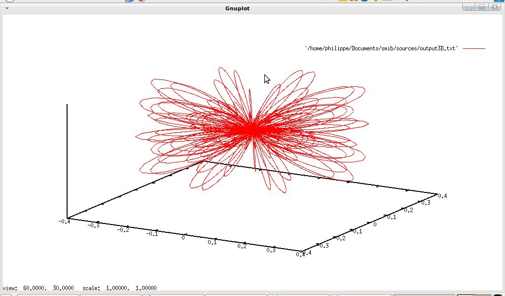
↓, one can use gnuplot3D and parametricsample, for example let plot3D.txt the file containing:
m=4
n=6
R=real(spherharm(theta,phi,m,n))
↓gnuplot3D(parametricsample(
(R*sin(theta)*cos(phi),R*sin(theta)*sin(phi),R*cos(theta))
,phi,theta,-4*pi,-pi,100))
quit()
In a terminal: ./smib ./plot3D.txt >> output3D.txt, so with qgfe:
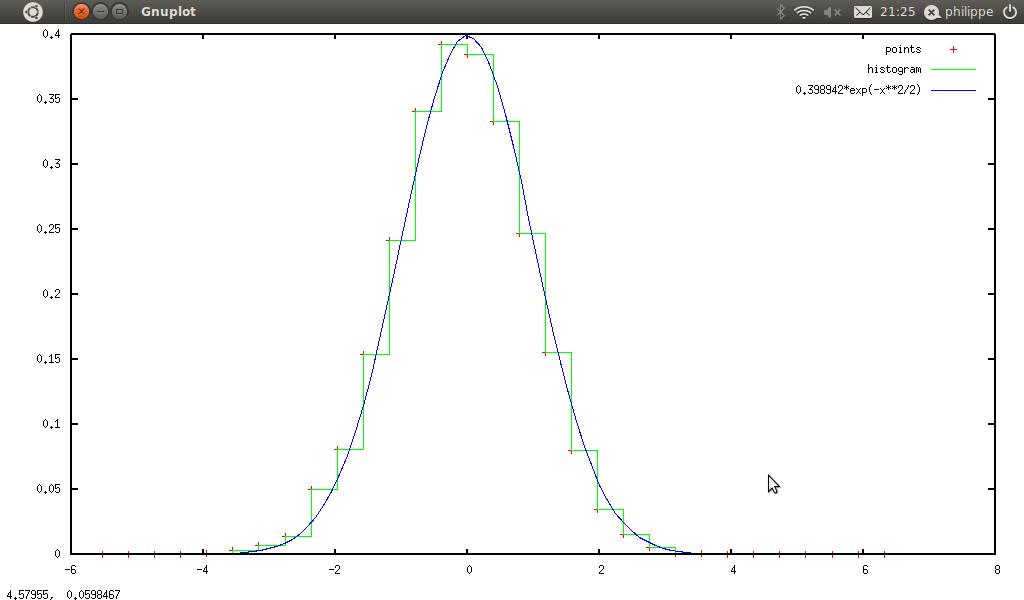
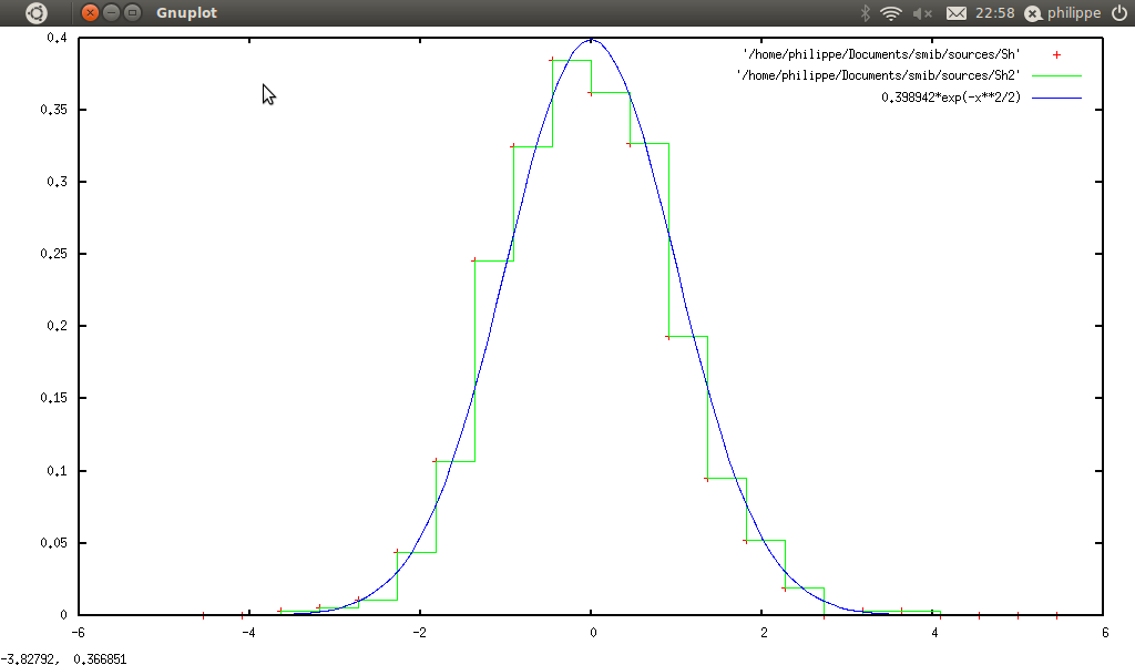
As we shall see later, qgfe is also useful to plot samples. We can use this feature to draw an histogram
↓s generated with smib. Here is a small example: we generate a large vector of normal random numbers (mean is null, variance is one), we compute the corresponding histogram, and then we compare this with the normal distribution. So in smib :
s=1
n=10000
Sr=normnoisevector(n,s)
Sh=Shistogram(Sr,I)
gnuplot2D(Sh)
quit()
And qgfe gives :
5 Applications
smib is certainly one of the smallest computer algebra system, but it is not a simple calculator. Here is the list of discussed topics discribed hereafter:
-
arithmetic & number theory:
-
primality tests
-
arithmetic functions properties
-
Dirichlet’s product properties
-
π computation
-
complex number and quaternion
-
function manipulation applied to quantum mechanic:
-
operator (creation, annihilation, commutator...)
-
operator acting on function
-
relation between quantum mechanic and Hermite function
-
differential geometry:
-
theory of curves: planar & 3D
-
gaussian theory of surfaces
-
riemannian geometry
-
unidimensional calculus:
-
classical integrals
-
orthogonal polynomial properties
-
complex path integrals
-
continous Fourier transform:
-
elementary functions
-
Fourier transform & convolution product
-
Fourier transform & Green functions
-
vectorial calculus:
-
vectorial integrals
-
curvilinear integrals
-
area integrals
-
Green theorem
-
Stokes theorem
-
Gauss-Ostrogradski theorem
-
numerical analysis:
-
univariate calculus applied to samples
-
special function (Bessel, Hankel, Airy...)
-
interpolation (Lagrange-Newton, least squares mean)
-
polynomial interpolation
-
numerical integration
-
discrete Fourier transform using samples:
-
elementary functions
-
differential equations
-
pseudo-differential operator
-
wavelets
-
complex analysis
-
ordinary differential equation
-
fractional calculus
-
probability & statistic:
-
distributions
-
moments
-
quantile & median
-
random numbers generation
-
law of large numbers & central limit theorem
-
stochastic differential equation
5.1 Arithmetic, Number theory & Polynomial
5.1.1 Computing famous numbers
Using direct computation
If one wants to compute
↓Mersenne number
↓ using
Mn = 2n − 1, one must define a function:
mersenneN(n)=2^n-1
then mersenneN(10) gives 1023.
Using recursive computation
To compute
↓↓Fibonacci number using
F0 = 0, F1 = 1, Fn = Fn − 1 + Fn − 2, so in smib:
fibonacciN(n)=test(n==0,0,test(n==1,1,fibonacciN(n-1)+fibonacciN(n-2)))
then fibonacciN(10) gives 55.
Using generating function
↓Bernoulli numbers
↓ Bn are defined as
x⁄ex − 1 = ∑n = ∞n = 0Bnxn⁄n!, in smib:
bernoulliN(n)=prog(temp,test(n==0,1,
limit(temp^(-n)*taylor(temp/(exp(temp)-1),temp,n,0)*n!,temp,infty)))
then bernoulliN(1) gives -1/2 or bernoulliN(10) gives 5/66.
5.1.2 ↓primality tests
↓Deterministic test: using ↓Wilson formula↓
This test is very simple to implement:
wilson(n)=test(mod((n-1)!+1,n)==0,1,0)
then wilson(1111) gives 0, and wilson(13) gives 1.
↓Probabilistic test: ↓Solovay-Strassen test
This test is harder to implement:
solovaystrassen(n,k)=prog(temp0,temp1,temp2,temp3,temp4,do(
temp1=0,
temp4=1,
test(iseven(n)==1,temp4=0,
for(temp0,1,k,
do(temp2=ceiling(random()*(n-1)),
test(iseven(temp2)==1,temp2=temp2+1),
temp3=jacobisymbol(n,temp2)*(-1)^((n-1)(temp2-1)/4),
test(or(temp3==0,not(mod(temp2^((n-1)/2)-temp3,n)==0)),
do(temp4=0,temp0=k))))),
return(temp4)
))
Here, we must use law of quadratic reciprocity for ↓Jacobi symbol↓ (this is due to Jacobi symbol definition in smib: it is stupid to compute decomposition into prime factors to test primality of a number).
Then solovaystrassen(761,14) gives 1 and solovaystrassen(763,14) gives 0.
In fact, those algorithmes are not very efficient in smib for large integers, it is better to use the function ↓isprime.
5.1.3 properties of arithmetic functions↓↓
Let X = (1, 2, 3, 4, 20, 25, 154, 210, 576, 6930, 22464, 54000, 104729, 193440, 523567) a vector of integers. Our aim is to test properties of arithmetic functions on this vector.
↓Sum over divisors
Here is the list of properties:
-
∑d|N|μ(d)|φ(d) = γ(N)
-
∑d|N1⁄d2 = σ(N, 2)⁄N2
-
∑d|N|μ(d)| = 2ω(N)
-
∑d|Nμ(d)τ(d) = ( − 1)ω(N)
-
∑d|Nμ(d)λ(d) = 2ω(N)
-
∑d|Nσ(d, 1) = N.∑d|Nτ(d)⁄d
The implementation is given by:
print("* a * Sum((n<=N,n|N),(|mu(n)|.phi(n)))=gamma(n) *")
testa(N)=sumoverdivisor(x,N,quote(abs(mobius(x))*eulerphi(x)))-integerkernel(N)
for(ind,1,dim(X),
print("Sum((n<=",X[ind],",n|N),(|mu|.phi))-gamma(",X[ind],")=",
testa(X[ind])))
print("* b * Sum((n<=N,n|N),1/n^2)=sigma(N,2)/N^2 *")
testb(N)=sumoverdivisor(x,N,1/x^2)-sigma(N,2)/N^2
for(ind,1,dim(X),
print("Sum((n<=",X[ind],",n|N),1/n^2)-sigma(",X[ind],",2)/",X[ind],"^2)=",
testb(X[ind])))
print("* c * Sum((n<=N,n|N),abs(mu(n)))=2^omega(n) *")
testc(N)=sumoverdivisor(x,N,quote(abs(mobius(x))))-2^omega(N)
for(ind,1,dim(X),
print("Sum((n<=",X[ind],",n|N),abs(mu(n)))-2^omega(",X[ind],")= ",
testc(X[ind])))
print("* d * Sum((n<=N,n|N),mu(n)*tau(n))=(-1)^omega(n) *")
testd(N)=sumoverdivisor(x,N,quote(mobius(x)*tau(x)))-(-1)^omega(N)
for(ind,1,dim(X),
print("Sum((n<=",X[ind],",n|N),mu(n)*tau(n))-
(-1)^omega(",X[ind],") = ",testd(X[ind])))
print("* e * Sum((n<=N,n|N),mu(n)*lamba(n))=2^omega(n) *")
teste(N)=sumoverdivisor(x,N,quote(mobius(x)*liouvillefunction(x)))-2^omega(N)
for(ind,1,dim(X),
print("Sum((n<=",X[ind],",n|N),mobius(n)*liouvillefunction(n))-
2^omega(",X[ind],") = ",teste(X[ind])))
print("* f * Sum((n<=N,n|N),sigma(n))=N*Sum((n<=N,n|N),tau(n)/n) *")
testf(N)=sumoverdivisor(x,N,quote(sigma(x,1)))-N*sumoverdivisor(x,N,quote(tau(x)/x))
for(ind,1,dim(X),
print("Sum((n<=",X[ind],",n|N),sigma(n,1))-Sum((n<=",X[ind],"n|N),
tau(n)/n) = ",testf(X[ind])))
And smib gives:
* a * Sum((n<=N,n|N),(|mu(n)|.phi(n)))=gamma(n) *
Sum((n<= 1 ,n|N),(|mu|.phi))-gamma( 1 ) = 0
Sum((n<= 2 ,n|N),(|mu|.phi))-gamma( 2 ) = 0
Sum((n<= 3 ,n|N),(|mu|.phi))-gamma( 3 ) = 0
Sum((n<= 4 ,n|N),(|mu|.phi))-gamma( 4 ) = 0
Sum((n<= 20 ,n|N),(|mu|.phi))-gamma( 20 ) = 0
Sum((n<= 25 ,n|N),(|mu|.phi))-gamma( 25 ) = 0
Sum((n<= 154 ,n|N),(|mu|.phi))-gamma( 154 ) = 0
Sum((n<= 210 ,n|N),(|mu|.phi))-gamma( 210 ) = 0
Sum((n<= 576 ,n|N),(|mu|.phi))-gamma( 576 ) = 0
Sum((n<= 6930 ,n|N),(|mu|.phi))-gamma( 6930 ) = 0
Sum((n<= 22464 ,n|N),(|mu|.phi))-gamma( 22464 ) = 0
Sum((n<= 54000 ,n|N),(|mu|.phi))-gamma( 54000 ) = 0
Sum((n<= 104729 ,n|N),(|mu|.phi))-gamma( 104729 ) = 0
Sum((n<= 193440 ,n|N),(|mu|.phi))-gamma( 193440 ) = 0
Sum((n<= 523567 ,n|N),(|mu|.phi))-gamma( 523567 ) = 0
* b * Sum((n<=N,n|N),1/n^2)=sigma(N,2)/N^2 *
Sum((n<= 1 ,n|N),1/n^2)-sigma( 1 ,2)/ 1 ^2) = 0
Sum((n<= 2 ,n|N),1/n^2)-sigma( 2 ,2)/ 2 ^2) = 0
Sum((n<= 3 ,n|N),1/n^2)-sigma( 3 ,2)/ 3 ^2) = 0
Sum((n<= 4 ,n|N),1/n^2)-sigma( 4 ,2)/ 4 ^2) = 0
Sum((n<= 20 ,n|N),1/n^2)-sigma( 20 ,2)/ 20 ^2) = 0
Sum((n<= 25 ,n|N),1/n^2)-sigma( 25 ,2)/ 25 ^2) = 0
Sum((n<= 154 ,n|N),1/n^2)-sigma( 154 ,2)/ 154 ^2) = 0
Sum((n<= 210 ,n|N),1/n^2)-sigma( 210 ,2)/ 210 ^2) = 0
Sum((n<= 576 ,n|N),1/n^2)-sigma( 576 ,2)/ 576 ^2) = 0
Sum((n<= 6930 ,n|N),1/n^2)-sigma( 6930 ,2)/ 6930 ^2) = 0
Sum((n<= 22464 ,n|N),1/n^2)-sigma( 22464 ,2)/ 22464 ^2) = 0
Sum((n<= 54000 ,n|N),1/n^2)-sigma( 54000 ,2)/ 54000 ^2) = 0
Sum((n<= 104729 ,n|N),1/n^2)-sigma( 104729 ,2)/ 104729 ^2) = 0
Sum((n<= 193440 ,n|N),1/n^2)-sigma( 193440 ,2)/ 193440 ^2) = 0
Sum((n<= 523567 ,n|N),1/n^2)-sigma( 523567 ,2)/ 523567 ^2) = 0
* c * Sum((n<=N,n|N),abs(mu(n)))=2^omega(n) *
Sum((n<= 1 ,n|N),abs(mu(n)))-2^omega( 1 ) = 0
Sum((n<= 2 ,n|N),abs(mu(n)))-2^omega( 2 ) = 0
Sum((n<= 3 ,n|N),abs(mu(n)))-2^omega( 3 ) = 0
Sum((n<= 4 ,n|N),abs(mu(n)))-2^omega( 4 ) = 0
Sum((n<= 20 ,n|N),abs(mu(n)))-2^omega( 20 ) = 0
Sum((n<= 25 ,n|N),abs(mu(n)))-2^omega( 25 ) = 0
Sum((n<= 154 ,n|N),abs(mu(n)))-2^omega( 154 ) = 0
Sum((n<= 210 ,n|N),abs(mu(n)))-2^omega( 210 ) = 0
Sum((n<= 576 ,n|N),abs(mu(n)))-2^omega( 576 ) = 0
Sum((n<= 6930 ,n|N),abs(mu(n)))-2^omega( 6930 ) = 0
Sum((n<= 22464 ,n|N),abs(mu(n)))-2^omega( 22464 ) = 0
Sum((n<= 54000 ,n|N),abs(mu(n)))-2^omega( 54000 ) = 0
Sum((n<= 104729 ,n|N),abs(mu(n)))-2^omega( 104729 ) = 0
Sum((n<= 193440 ,n|N),abs(mu(n)))-2^omega( 193440 ) = 0
Sum((n<= 523567 ,n|N),abs(mu(n)))-2^omega( 523567 ) = 0
* d * Sum((n<=N,n|N),mu(n)*tau(n))=(-1)^omega(n) *
Sum((n<= 1 ,n|N),mu(n)*tau(n))-(-1)^omega( 1 ) = 0
Sum((n<= 2 ,n|N),mu(n)*tau(n))-(-1)^omega( 2 ) = 0
Sum((n<= 3 ,n|N),mu(n)*tau(n))-(-1)^omega( 3 ) = 0
Sum((n<= 4 ,n|N),mu(n)*tau(n))-(-1)^omega( 4 ) = 0
Sum((n<= 20 ,n|N),mu(n)*tau(n))-(-1)^omega( 20 ) = 0
Sum((n<= 25 ,n|N),mu(n)*tau(n))-(-1)^omega( 25 ) = 0
Sum((n<= 154 ,n|N),mu(n)*tau(n))-(-1)^omega( 154 ) = 0
Sum((n<= 210 ,n|N),mu(n)*tau(n))-(-1)^omega( 210 ) = 0
Sum((n<= 576 ,n|N),mu(n)*tau(n))-(-1)^omega( 576 ) = 0
Sum((n<= 6930 ,n|N),mu(n)*tau(n))-(-1)^omega( 6930 ) = 0
Sum((n<= 22464 ,n|N),mu(n)*tau(n))-(-1)^omega( 22464 ) = 0
Sum((n<= 54000 ,n|N),mu(n)*tau(n))-(-1)^omega( 54000 ) = 0
Sum((n<= 104729 ,n|N),mu(n)*tau(n))-(-1)^omega( 104729 ) = 0
Sum((n<= 193440 ,n|N),mu(n)*tau(n))-(-1)^omega( 193440 ) = 0
Sum((n<= 523567 ,n|N),mu(n)*tau(n))-(-1)^omega( 523567 ) = 0
* e * Sum((n<=N,n|N),mu(n)*lamba(n))=2^omega(n) *
Sum((n<= 1 ,n|N),mobius(n)*liouvillefunction(n))-2^omega( 1 ) = 0
Sum((n<= 2 ,n|N),mobius(n)*liouvillefunction(n))-2^omega( 2 ) = 0
Sum((n<= 3 ,n|N),mobius(n)*liouvillefunction(n))-2^omega( 3 ) = 0
Sum((n<= 4 ,n|N),mobius(n)*liouvillefunction(n))-2^omega( 4 ) = 0
Sum((n<= 20 ,n|N),mobius(n)*liouvillefunction(n))-2^omega( 20 ) = 0
Sum((n<= 25 ,n|N),mobius(n)*liouvillefunction(n))-2^omega( 25 ) = 0
Sum((n<= 154 ,n|N),mobius(n)*liouvillefunction(n))-2^omega( 154 ) = 0
Sum((n<= 210 ,n|N),mobius(n)*liouvillefunction(n))-2^omega( 210 ) = 0
Sum((n<= 576 ,n|N),mobius(n)*liouvillefunction(n))-2^omega( 576 ) = 0
Sum((n<= 6930 ,n|N),mobius(n)*liouvillefunction(n))-2^omega( 6930 ) = 0
Sum((n<=22464,n|N),mobius(n)*liouvillefunction(n))-2^omega( 22464 ) = 0
Sum((n<=54000,n|N),mobius(n)*liouvillefunction(n))-2^omega( 54000 ) = 0
Sum((n<=104729,n|N),mobius(n)*liouvillefunction(n))-2^omega(104729) = 0
Sum((n<=193440,n|N),mobius(n)*liouvillefunction(n))-2^omega(193440) = 0
Sum((n<=523567,n|N),mobius(n)*liouvillefunction(n))-2^omega(523567) = 0
* f * Sum((n<=N,n|N),sigma(n))=N*Sum((n<=N,n|N),tau(n)/n) *
Sum((n<= 1 ,n|N),sigma(n,1))-Sum((n<= 1 n|N),tau(n)/n) = 0
Sum((n<= 2 ,n|N),sigma(n,1))-Sum((n<= 2 n|N),tau(n)/n) = 0
Sum((n<= 3 ,n|N),sigma(n,1))-Sum((n<= 3 n|N),tau(n)/n) = 0
Sum((n<= 4 ,n|N),sigma(n,1))-Sum((n<= 4 n|N),tau(n)/n) = 0
Sum((n<= 20 ,n|N),sigma(n,1))-Sum((n<= 20 n|N),tau(n)/n) = 0
Sum((n<= 25 ,n|N),sigma(n,1))-Sum((n<= 25 n|N),tau(n)/n) = 0
Sum((n<= 154 ,n|N),sigma(n,1))-Sum((n<= 154 n|N),tau(n)/n) = 0
Sum((n<= 210 ,n|N),sigma(n,1))-Sum((n<= 210 n|N),tau(n)/n) = 0
Sum((n<= 576 ,n|N),sigma(n,1))-Sum((n<= 576 n|N),tau(n)/n) = 0
Sum((n<= 6930 ,n|N),sigma(n,1))-Sum((n<= 6930 n|N),tau(n)/n) = 0
Sum((n<= 22464 ,n|N),sigma(n,1))-Sum((n<= 22464 n|N),tau(n)/n) = 0
Sum((n<= 54000 ,n|N),sigma(n,1))-Sum((n<= 54000 n|N),tau(n)/n) = 0
Sum((n<= 104729 ,n|N),sigma(n,1))-Sum((n<= 104729 n|N),tau(n)/n) = 0
Sum((n<= 193440 ,n|N),sigma(n,1))-Sum((n<= 193440 n|N),tau(n)/n) = 0
Sum((n<= 523567 ,n|N),sigma(n,1))-Sum((n<= 523567 n|N),tau(n)/n) = 0
Product over divisors↓ (or prime divisors↓)
Here is the list of properties:
-
∏d|Nd = N.τ(N)⁄2
-
( − 1)ω(N)∏p|Np = ∑d|Nμ(d)σ(d, 1)
-
( − 1)ω(N)∏p|N(p − 2) = ∑d|Nμ(d)φ(d).
The implementation is:
print("* a * product((n<=N,n|N),n)=N^(tau(N)/2) *")
testa(N)=productoverdivisor(x,N,quote(x))-N^(tau(N)/2)
for(ind,1,dim(X),print("Product((n<=",X[ind],",n|N),n)-
",X[ind],"^(tau(",X[ind],")/2) =",testa(X[ind])))
print("* b * (-1)^omega(N)*product((n<=N,isprime(n)),n)=
Sum((n<=N,n|N),mu(n)*sigma(n)) *")
testb(N)=(-1)^omega(N)*productoverprime(x,N,x)-
sumoverdivisor(x,N,quote(mobius(x)*sigma(x,1)))
for(ind,1,dim(X),print("(-1)^omega(",X[ind],")*Product((n<=",X[ind],",
isprime(n)), n)-Sum((n<=",X[ind],",n|N),mu(n)*sigma(n)) =",testb(X[ind])))
print("* c * (-1)^omega(N)*product((n<=N,isprime(n)),n-2)=
Sum((n<=N,n|N),mu(n)*phi(n)) *")
testc(N)=(-1)^omega(N)*productoverprime(x,N,x-2)-
sumoverdivisor(x,N,quote(mobius(x)*eulerphi(x)))
for(ind,1,dim(X),print("(-1)^omega(",X[ind],")*Product((n<=",X[ind],",
isprime(n)), n-2)-Sum((n<=",X[ind],",n|N),mu(n)*phi(n)) =",testc(X[ind])))
And smib gives:
↓↓Dirichlet product
Here is the list of properties of Dirichlet product:
-
σ = id⋆1
-
τ = 1⋆1
-
φ = μ⋆id
-
σ = φ⋆τ
-
id = σ⋆μ
-
id = φ⋆1
-
id.τ = φ⋆σ
-
(id.σ)(n) = ∑d|nτ(d)
-
(id2.σ)(n) = ∑d|nd.σ(d)
-
σ⋆σ = (id.τ)⋆τ
-
∑1≤n≤N(τ⋆μ⋆Λ)(n) = log(N!)(here X = (1, 2, 3, 4, 20, 25, 154))
And implementation is given by:
print("* a * sigma = id * 1 *")
Sigma(n)=dirichletproduct(1,x,x,n)
for(ind,1,dim(X),print("Sigma(",X[ind],",1)-(id*1)(",X[ind],")=",
Sigma(X[ind])-sigma(X[ind],1)))
print("* b * phi = mu * id *")
phi(n)=dirichletproduct(quote(mobius(x)),x,x,n)
for(ind,1,dim(X),print("phi(",X[ind],")-(mu*id)(",X[ind],")=",
phi(X[ind])-eulerphi(X[ind])))
print("* c * sigma = tau * phi *")
tau(n)=dirichletproduct(1,1,x,n)
sigma2(n)=dirichletproduct(quote(tau(x)),quote(eulerphi(x)),x,n)
for(ind,1,dim(X),print("sigma(",X[ind],")-(tau*phi)(",X[ind],",1)=",
sigma2(X[ind])-sigma(X[ind],1)))
print("* d * id = sigma * mu *")
testd(n)=dirichletproduct(quote(sigma(x,1)),quote(mobius(x)),x,n)-n
for(ind,1,dim(X),print("id(",X[ind],")-(sigma*mu)(",X[ind],")=",
testd(X[ind])))
print("* e * id = phi * 1 *")
teste(n)=dirichletproduct(1,quote(eulerphi(x)),x,n)-n
for(ind,1,dim(X),print("id(",X[ind],")-(phi*1)(",X[ind],")=",teste(X[ind])))
print("* f * id tau = phi * sigma *")
testf(n)=dirichletproduct(quote(eulerphi(x)),quote(sigma(x,1)),x,n)-n*tau(n)
for(ind,1,dim(X),print("id tau(",X[ind],")-(phi*sigma)(",X[ind],")=",
testf(X[ind])))
print("* g * id*sigma(n) = Sum((n<=N,n|N),n tau(n)) *")
testg(n)=dirichletproduct(quote(x),quote(sigma(x,1)),x,n)
sumoverdivisor(x,n,quote(x*tau(x)))
for(ind,1,dim(X),print("(id*sigma)(",X[ind],")-
Sum((n<=",X[ind],"n|N),n*tau(n))=",testg(X[ind])))
print("* h * id^2*sigma(n) = Sum((n<=N,n|N),n sigma(n)) *")
testh(n)=dirichletproduct(quote(x^2),quote(sigma(x,1)),x,n)-
sumoverdivisor(x,n,quote(x*sigma(x,1)))
for(ind,1,dim(X),print("(id^2*sigma)(",X[ind],")-
Sum((n<=",X[ind],"n|N),n*sigma(n))=",testh(X[ind])))
print("* i * sigma*sigma(n) = (id tau)*tau *")
testi(n)=dirichletproduct(quote(sigma(x,1)),quote(sigma(x,1)),x,n)-
dirichletproduct(quote(x*tau(x)),quote(tau(x)),x,n)
for(ind,1,dim(X),print("(sigma*sigma-(id tau)*tau)(",X[ind],")=",
testi(X[ind])))
X=(1,2,3,4,20,25,154)
print("* j * Sum(n<=N,(tau(n)*mu(n)*lambda(n)))=log(N!) *")
testj(N)=sum(ind,1,N,dirichletproduct(dirichletproduct(quote(tau(x)),
quote(mobius(x)),x,ind),quote(mangoldt(x)),x,ind))-log(N!)
for(ind,1,dim(X),print("Sum(n<=",X[ind],",(tau*mu*lambda)-
log(",X[ind],"!) =",num(testj(X[ind]))))
And smib gives:
5.1.4 ↓↓Arithmetic equations
Here, we want to solve the following equation:
⎛⎜⎝
x
n
⎞⎟⎠ + ⎛⎜⎝
y
n
⎞⎟⎠ = ⎛⎜⎝
z
n
⎞⎟⎠, n≥3, x, y, z≤20.
So in smib:
i=1
for(n,3,5,
for(x,n,20,
for(y,n,20,
for(z,n,20,
test(binomial(x,n)+binomial(y,n)-binomial(z,n)==0,
do(print("solution: ",i),
print("n=",n),
print("x=",x),
print("y=",y),
print("z=",z),
i=i+1
))))))
And the result is:
solution: 1
n= 3
x= 5
y= 5
z= 6
solution: 2
n= 3
x= 10
y= 16
z= 17
solution: 3
n= 3
x= 16
y= 10
z= 17
solution: 4
n= 4
x= 7
y= 7
z= 8
solution: 5
n= 5
x= 9
y= 9
z= 10
-
4τ(n + 2) = φ(n), 0≤n≤1000
So simply in smib:
for(n,1,1000, test(4*tau(n+2)-eulerphi(n)==0,print(n)))
And the result is:
15
32
60
64
68
90
102
110
130
-
σ(n, 1) = 2n + 1, 0≤n≤1000
So simply in smib:
for(n,1,1000, test(sigma(n,1)-2*n+1==0,print(n)))
And the result is:
1
2
4
8
16
32
64
128
256
512
In fact we can show that σ(n, 1) = 2n + 1 ⇔ n = 2m
5.1.5 Perfect number↓ & harmonic mean of divisors↓
An positive integer is perfect if it is equal to the sum of its proper positive divisors. This definition is equivalent to :
n is perfect
⟺σ(n, 1) = 2n.
So in smib :
isperfect(n,k)=test(sigma(n,1)==k*n,1,0)
The harmonic mean of divisors of a positive integer is defined as : H(n) = τ(n)⁄∑d|n1⁄d.
So in smib : harmonicmean(n)=tau(n)/sumoverdivisor(x,n,1/x)
Perfection and harmonic mean of divisors are linked by the following property :
n is perfect ⟺2H(n) − 1(2H(n) − 1) = n.
How many perfect numbers are between 0 and 10000?
So in smib using isperfect :
test7(N)=test(isperfect(N,2)==1,print(N))
for(ind,1,10000,test7(ind))
So smib gives :
6
28
496
8128
So in smib using property of harmonic mean :
test8(N)=prog(H,do(H=harmonicmean(N),
test(2^(H-1)*(2^H-1)==N,print(N))))
for(ind,1,10000,test8(ind))
So smib gives :
6
28
496
8128
N.B. : computation time is very long...
5.1.6 Mertens function & Redheffer matrix
A
↓↓Redheffer matrix
R(n) is a matrix whose entries
aij are
1 if
i divides
j or if
j = 1; otherwise,
aij = 0. So in smib :
redheffer(n)=prog(indi,indj,tabA,val,do(
tabA=zero(n,n),
for(indi,1,n,
for(indj,1,n,
do(test(or(indj==1,mod(indj,indi)==0),val=1,val=0),
tabA[indi,indj]=val))),
tabA
))
This matrix is linked to Mertens function↓↓ by the following relation :M(n) = det(R(n)), we are going to test it, so in smib :
n=5
A=redheffer(n)
print("A = ",A)
print("det(A) = ",det(A))
print("mertens(n) = ",mertens(n))
And smib gives :
A = ((1,1,1,1,1),(1,1,0,1,0),(1,0,1,0,0),(1,0,0,1,0),(1,0,0,0,1))
det(A) = -2
mertens(n) = -2
5.1.7 Arithmetic & statistic
Let
A(n) be the set of
n first prime intergers, we want to study skewness
↓ and kurtosis
↓ of this set. In parallel, using prime number theorem, we can also study asymptotic behaviour of skewness and kurtosis. Using corollary of
↓prime number theorem, let
I(p, n) = 1⁄n∫n1[xln(x) − 1⁄n∫n1xln(x)dx]pdx, hence kurtosis is given by
ku(n) = I(4, n)⁄I(2, n)2 − 3, and skewness by
sk(n) = I(3, n)⁄I(2, n)3⁄2.
So in smib:
The next prime is define as:
nextprime(n)=test(isprime(n+1)==1,n+1,nextprime(n+1))
The set of n first primes:
listprime(n)=prog(temp,ind,do(
temp=zero(n),
for(ind,1,n,
test(ind==1,
temp[ind]=2,
temp[ind]=nextprime(temp[ind-1]))),
return(temp)))
And asymptotic behaviour by:
I(p,n)=1/n*defint((x*log(x)-1/n*defint(x*log(x),x,1,n))^p,x,1,n)
ku(n)=I(4,n)/I(2,n)^2-3
sk(n)=I(3,n)/I(2,n)^(3/2)
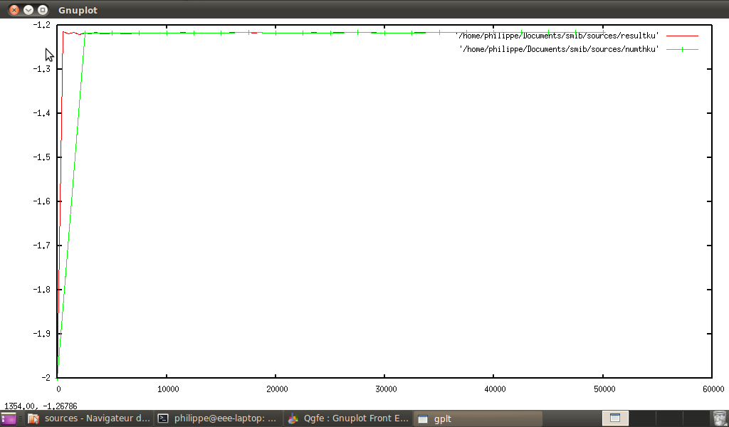
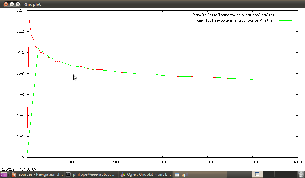
Now we can plot on same graphic:
-
statkurtosis(listprime(n)) and ku(n), and smib gives:
-
statskewness(listprime(n)) and sk(n), and smib gives:
In this paragraph, we will study some properties of polynomials in ℚ[x].
First we consider
↓↓euclidean division (
i.e. let
A, B ∈ ℚ[x] we want to find
Q, R ∈ ℚ[x] such that
A = BQ + R with
deg(R) < deg(B)), in smib we must use function
divpoly (this function can be used for multivariate polynomials too), hereafter three simple examples :
print("Euclidean division : A=B*Q+R , d°(R)<d°(B)")
A=3*x^3+x^2+x+5
B=5*x^2-3*x+1
D=divpoly(A,B,x)
print(A,"=",D[1],"*",B,"+",D[2])
A-(D[1]*B+D[2])
A=3*t*x^3+t^2*x^2+x+t^3*5
B=5*x^2-t*3*x+t
D=divpoly(A,B,x)
print(A,"=",D[1],"*",B,"+",D[2])
A-(D[1]*B+D[2])
D=divpoly(A,B,t)
print(A,"=",D[1],"*",B,"+",D[2])
A-(D[1]*B+D[2])
And smib gives :
Euclidean division : A=B*Q+R , d°(R)<d°(B)
5+x+x^2+3*x^3 = 14/25+3/5*x * 1-3*x+5*x^2 + 111/25+52/25*x
0
x+3*t*x^3+t^2*x^2+5*t^3 = 3/5*t*x+14/25*t^2 * t-3*t*x+5*x^2 +
x-3/5*t^2*x+42/25*t^3*x+111/25*t^3
0
x+3*t*x^3+t^2*x^2+5*t^3 =
-25*t*x^2/((1-3*x)^2)+t*x^2/(1-3*x)+5*t^2/(1-3*x)+
3*x^3/(1-3*x)+125*x^4/((1-3*x)^3)-5*x^4/((1-3*x)^2) * t-3*t*x+5*x^2 +
x+3*t*x^3-3*t*x^3/(1-3*x)-125*t*x^4/((1-3*x)^3)+130*t*x^4/((1-3*x)^2)+
4*t*x^4/(1-3*x)+375*t*x^5/((1-3*x)^3)-15*t*x^5/((1-3*x)^2)+t^2*x^2+
25*t^2*x^2/((1-3*x)^2)-26*t^2*x^2/(1-3*x)-75*t^2*x^3/((1-3*x)^2)+
3*t^2*x^3/(1-3*x)+15*t^3*x/(1-3*x)-5*t^3/(1-3*x)-15*x^5/(1-3*x)-
625*x^6/((1-3*x)^3)+25*x^6/((1-3*x)^2)+5*t^3
0
Now, using euclidean division, we can compute ↓greater common divisor (gcd) ↓ of two polynomials, in smib we must use function gcdpoly, a small example :
print("Euclidean algorithm : GCD")
A=x^4-2*x^3-6*x^2+12*x+15
B=x^3+x^2-4*x-4
D=gcdpoly(A,B,x)
D
temp=divpoly(A,D,x)[2]
test(temp==0,print("OK"),print("KO"))
temp=divpoly(B,D,x)[2]
test(temp==0,print("OK"),print("KO"))
And smib gives :
Euclidean algorithm : GCD
5 + 5 x
OK
OK
In the preceeding example, we compute D = gcd(A, B) and we verify that D divides A and D divides B.
Extended euclidean algorithm first version
Here we want to solve the following problem : let A, B ∈ ℚ[x] we want to find S, T, G ∈ ℚ[x] such that SA + TB = G, G = gcd(A, B), this problem is solved using extendedeuclidean. A small example :
a=x^4-2*x^3-6*x^2+12*x+15
b=x^3+x^2-4*x-4
D=extendedeuclidean(a,b,x)
print("s = ",D[1])
print("t = ",D[2])
print("g = ",D[3])
print("s*a+t*b-g = ",D[1]*a+D[2]*b-D[3])
And smib gives :
s = 3-x
t = 10-6*x+x^2
g = 5+5*x
s*a+t*b-g = 0
↓↓Extended euclidean algorithm second version
Here we generalized the preceeding problem : let A, B, C ∈ ℚ[x] we want to find S, T ∈ ℚ[x] such that SA + TB = C, this problem is solved using egcd. A small example :
a=x^4-2*x^3-6*x^2+12*x+15
b=x^3+x^2-4*x-4
c=x^2-1
D=egcd(a,b,c,x)
print("s = ",D[1])
print("t = ",D[2])
print("s*a+t*b-c = ",D[1]*a+D[2]*b-c)
And smib gives :
s = -3/5+4/5*x-1/5*x^2
t = -2+16/5*x-7/5*x^2+1/5*x^3
s*a+t*b-c = 0
N.B. : the solution exists if and only if C is in the ideal generated by A and B.
Half extended euclidean algorithm
Let A, B, C ∈ ℚ[x] we search S ∈ ℚ[x] such that SA ≡ C (mod B), to do this we use the function halfextendedeuclidean2. A small example :
a=x^4-2*x^3-6*x^2+12*x+15
b=x^3+x^2-4*x-4
c=x^2-1
D=halfextendedeuclidean2(a,b,c,x)
print("s = ",D)
print("s*a-c (mod b)= ",divpoly(D*a-c,b,x)[2])
And smib gives :
s = -3/5+4/5*x-1/5*x^2
s*a-c (mod b)= 0
Let A, B ∈ ℚ[x], we search S ∈ ℚ[x] such that SA ≡ 1 (mod B), this problem is solved using inversemod. Once again a small example :
a=x^4-2*x^3-6*x^2+12*x+15
b=x^2-4*x-4
D=inversemod(a,b,x)
print("D = ",D)
print("a^(-1)*a-1 (mod b) = ",divpoly(D*a-1,b,x)[2])
And smib gives :
D = 215/641-44/641*x
a^(-1)*a-1 (mod b) = 0
↓↓Chinese remainder theorem
Let Ai, Bi ∈ ℚ[x] with i ∈ {1, .., n}, n > 2, this time we search Xi ∈ ℚ[x] with i ∈ {1, .., n}, n > 2 such that Xi ≡ Ai (mod Bi), to do this we use the function chineserem its principal argument is a = (Ai, Bi)i ∈ {1, .., n}, n > 2. Hereafter three examples :
a=(((x+1)^2,x+1),((x-1)^3,x-1))
D=chineserem(a,x)
print(D)
for(ind,1,dim(a),print("D-a_i (mod b_i) = ", divpoly(D-a[ind,1],a[ind,2],x)[2]))
a=(((x+1)^2,x-1),((x-1)^3,x+1))
D=chineserem(a,x)
print(D)
for(ind,1,dim(a),print("D-a_i (mod b_i) = ", divpoly(D-a[ind,1],a[ind,2],x)[2]))
a=(((x+1)^2,x-1),((x-1)^3,x+1),((x+5)^2,x-2))
D=chineserem(a,x)
print(D)
for(ind,1,dim(a),print("D-a_i (mod b_i) = ", divpoly(D-a[ind,1],a[ind,2],x)[2]))
And smib gives :
3/2*x-1/2*x^2-3/2*x^3+1/2*x^4
D-a_i (mod b_i) = 0
D-a_i (mod b_i) = 0
7/2*x-3/2*x^2+5/2*x^3-1/2*x^4
D-a_i (mod b_i) = 0
D-a_i (mod b_i) = 0
-23/3+2/3*x+41/6*x^2+31/6*x^3-7/6*x^4+1/6*x^5
D-a_i (mod b_i) = 0
D-a_i (mod b_i) = 0
D-a_i (mod b_i) = 0
The factorization of a polynomial is a hard task, smib solves this partially, it is only able to compute square-free factorization
↓↓ using Yun algorithm
↓↓. Hereafter two small examples :
a=x^8+6*x^6+12*x^4+8*x^2
D=squarefreepoly(a,x)
print("Factorisation = ",D)
print(a-product(ind,1,dim(D),D[ind,1]^D[ind,2]))
a=x^8-5*x^6+6*x^4+4*x^2-8
D=squarefreepoly(a,x)
print("Factorisation = ",D)
print(a-product(ind,1,dim(D),D[ind,1]^D[ind,2]))
And smib gives :
Factorisation = ((x,2),(2+x^2,3))
0
Factorisation = ((1+x^2,1),(-2+x^2,3))
0
↓Field of rational functions
Let
A, B ∈ ℚ[x], if
B does not divide
A then
A⁄B∉ℚ[x], using some algebra we can construct the field of quotients which is denoted
ℚ(x). Using square-free decomposition of polynomials, we can compute the decomposition of rational function
↓↓ which is very useful to compute integral of rational function. A small example :
a=x^2+3*x
b=x^3-x^2-x+1
FD=fracred(a/b,x)
print("Frac = ",FD)
print("Frac-a/b = ",simplify(FD-a/b))
And smib gives :
Frac = 9*x/(4*(-1+x)^2)+3*x/(4*(1+x))+x^2/(4*(1+x))-x^3/(4*(-1+x)^2)
Frac-a/b = 0
N.B. : sometime this decomposition does not work because squarefreepoly is unable to compute factorization.
5.1.9 Sum↓ & Gosper algorithm↓↓
In this section, we want to study
∑n = bn = af(n), where
f is an hypergeometric function
↓↓ (i.e.
f(n + 1)⁄f(n) is a rational fraction). First, we consider
r(n) = f(n + 1)⁄f(n), then we search the polynomials
a,
b,
c, such that
r(n) = a(n)⁄b(n).c(n + 1)⁄c(n), then we search a polynomial
P such that
a(n)P(n + 1) − b(n − 1)P(n) = c(n). Then
∑k = n − 1k = 0f(k) = b(n − 1)⁄c(n)x(n).f(n) = g(n),
g is the antidifference
↓ of
f. Finally, \strikeout off\uuline off\uwave off
∑n = bn = af(n) = g(b + 1) − g(a).
As usual there are some
↓weaknesses :
f must be factorizable over integer, and
deg(P) < 10.
Some examples :
∑n1⁄(n(n + 1)) ,
∑n1⁄(n(n + 1)(n + 2)) ,
∑nn2,
∑nann2,
∑n2nn2,
∑n(4n + 1)n!⁄(2n + 1)!
verbmode=0
f=1/(n*(n+1))
print("f = ",f)
verbmode=1
print("antidiff = ",simfac(factor(gosper(f,n))))
verbmode=0
print("Sum = ",gospersum(f,n,1,m))
print("Limit = ",limit(gospersum(f,n,1,m),m,infty))
f=1/(n*(n+1)*(n+2))
print("f = ",f)
print("antidiff = ",simfac(factor(gosper(f,n))))
print("Sum = ",gospersum(f,n,3,m))
print("Limit = ",limit(gospersum(f,n,1,m),m,infty))
f=n^2
print("f = ",f)
verbmode=1
print("antidiff = ",simfac(factor(gosper(f,n))))
verbmode=0
print("Sum = ",gospersum(f,n,0,m))
f=a^n*n^2
print("f = ",f)
print("antidiff = ",simfac(factor(gosper(f,n))))
print("Sum = ",gospersum(f,n,0,m))
f=2^n*n^2
print("f = ",f)
print("antidiff = ",simfac(factor(gosper(f,n))))
print("Sum = ",gospersum(f,n,0,m))
f=(4*n+1)*n!/(2*n+1)!
print("f = ",f)
print("antidiff = ",simfac(factor(gosper(f,n))))
print("Sum = ",gospersum(f,n,0,m))
f=n*n!
print("f = ",f)
print("antidiff = ",simfac(factor(gosper(f,n))))
print("Sum = ",gospersum(f,n,0,m))
f=n!
simfac(factor(gosper(f,n)))
gospersum(f,n,0,m)
And smib gives :
f = 1/(n*(1+n))
antidiff =
Gosper : t( n ) = 1/(n*(1+n))
f = t( 1+n )/t( n ) = n/(2+n)
GCD = -2
Numf = n
Denomf = 2+n
dimDecomp = 0
DecompDenom = 2+n
divtemp1 = (1,0)
divtemp2 = (1,-3)
an = n
bn = 2+n
cn = 1
CTRL 1 = 0
degree(an,n)==degree(bn,n)
leadingcoeff(an,n)==leadingcoeff(bn,n)
degdec = 0
EGCD = (-1,-1)
CTRL 2 = 0
-1/n
Sum = m/(1+m)
Limit = 1
f = 1/(n*(1+n)*(2+n))
antidiff = -1/(2*n*(1+n))
Sum = (-5-1/6*m+m^2+1/6*m^3)/(4*(6+11*m+6*m^2+m^3))
Limit = 1/4
f = n^2
antidiff =
Gosper : t( n ) = n^2
f = t( 1+n )/t( n ) = (1+2*n+n^2)/(n^2)
GCD = 1/4
Numf = 1+2*n+n^2
Denomf = n^2
dimDecomp = 0
DecompDenom = n^2
divtemp1 = (1,0)
divtemp2 = (1,0)
an = 1
bn = 1
cn = n^2
CTRL 1 = 0
degree(an,n)==degree(bn,n)
leadingcoeff(an,n)==leadingcoeff(bn,n)
degdec = 3
V = (0,-1,-4,-9)
MVhomo = (-a1-a2-a3,-a1-3*a2-7*a3,-a1-5*a2-19*a3,-a1-7*a2-37*a3)
M = ((0,-1,-1,-1),(0,-1,-3,-7),(0,-1,-5,-19),(0,-1,-7,-37))
M = ((-1,-3,-7),(-1,-5,-19),(-1,-7,-37))
V = (-1,-4,-9)
Sol = (1/6,-1/2,1/3)
V[1]==0
P = n*(1/6-1/2*n+1/3*n^2)
CTRL 2 = 0
1/6*n*(-1+n)*(-1+2*n)
Sum = m*(1/6+1/2*m+1/3*m^2)
f = a^n*n^2
antidiff = a^n*(-1+a)^6*
(-a-2*a*n+2*a*n^2+2*a^2*n-a^2*n^2-a^2-n^2)/
(1-9*a+36*a^2-84*a^3+126*a^4-126*a^5+84*a^6-36*a^7+9*a^8-a^9)
Sum = (a-2*a^(1+m)*m-a^(1+m)*m^2+14*a^(2+m)*m+8*a^(2+m)*
m^2-42*a^(3+m)*m-28*a^(3+m)*m^2+70*a^(4+m)*m+56*a^(4+m)*
m^2-70*a^(5+m)*m-70*a^(5+m)*m^2+42*a^(6+m)*m+56*a^(6+m)*
m^2-14*a^(7+m)*m-28*a^(7+m)*m^2+2*a^(8+m)*m+8*a^(8+m)*
m^2-a^(9+m)*m^2-5*a^2+9*a^3-5*a^4-5*a^5+9*a^6-5*a^7+a^8-
a^(1+m)+5*a^(2+m)-9*a^(3+m)+5*a^(4+m)+5*a^(5+m)-9*a^(6+m)+
5*a^(7+m)-a^(8+m))/(1-9*a+36*a^2-84*a^3+126*a^4-126*a^5+
84*a^6-36*a^7+9*a^8-a^9)
f = 2^n*n^2
antidiff = 2^n*(6-4*n+n^2)
Sum = -6-2*2^(1+m)*m+2^(1+m)*m^2+3*2^(1+m)
f = 4*n*n!/(1+2*n)!+n!/(1+2*n)!
antidiff = -2*n!/(2*n)!
Sum = (-15*(1+m)!+5*(3+2*m)!-22*m*(1+m)!+4*m*(3+2*m)!-8*m^2*(1+m)!)
/((5/2+2*m)*(1+2*0)!*(1+2*(1+m))!)
f = n*n!
antidiff = gosper failed Stop: user stop
5.2 Unidimensional integral↓ calculus↓
In this chapter, we wants to show how to use symbolic computation of antiderivative (using the function antider) or of definite integrals (using the function defint).
5.2.1 ↓Antiderivative
We want to solve this problem : for a given function
f find
F such that
F’ = f. This problem is solved using the function
antider↓, it handles polynomials↓, rational functions↓↓, functions like c.g’(x).h(g(x)) where c is a constant, g is a fonction, h is a power function, trigonometric (or inverse trigonometric) function↓↓↓↓,↓↓↓↓ hyperbolic trigonometric (or inverse hyperbolic trigonometric) function, ↓↓exponential or ↓↓logarithmic fuction, or derivative of those functions.
Hereafter some examples (those examples are as usual in tutorial):
N.B. :
-
In the directory /smib/documentation/application/Performance, we find the file testintegral which contains about 300 integrals, at the moment smib gives a good answer at 92% at least.
-
we are very far from Risch algorithm↓.
5.2.2 Classical integrals
Here is a list of classical integrals:
-
∫[ − ∞, ∞]1[a, b]dx
-
∬[a1, b1] × [a2, b2]1dx
-
∫[ − ∞, ∞]e − x2dx
-
∫[ − ∞, ∞]1⁄(1 + x2)dx
-
∫[0, ∞]sin(x)⁄xdx
-
∫[ − ∞, ∞]sin(x)⁄xdx
-
∫[0, ∞]e − xdx.
The implementation is given by:
print("defint(carac(x,a,b),x,minfty,infty)=",
defint(carac(x,a,b),x,minfty,infty))
print("defint(defint(1,x,a1,b1),y,a2,b2)=",
defint(defint(1,x,a1,b1),y,a2,b2))
print("defint(exp(-x^2),x,minfty,infty)=",
defint(exp(-x^2),x,minfty,infty))
print("defint(1/(1+x^2),x,minfty,infty)=",
defint(1/(1+x^2),x,minfty,infty))
print("defint(sin(x)/x,x,0,infty)=",
defint(sin(x)/x,x,0,infty))
print("defint(sin(x)/x,x,minfty,infty)=",
defint(sin(x)/x,x,minfty,infty))
print("defint(exp(-x),x,0,infty)=",
defint(exp(-x),x,0,infty))
And smib gives:
defint(carac(x,a,b),x,minfty,infty)= -a+b
defint(defint(1,x,a1,b1),y,a2,b2)= a1*a2-a1*b2-a2*b1+b1*b2
defint(exp(-x^2),x,minfty,infty)= pi^(1/2)
defint(1/(1+x^2),x,minfty,infty)= pi
defint(sin(x)/x,x,0,infty)= 1/2*pi
defint(sin(x)/x,x,minfty,infty)= pi
defint(exp(-x),x,0,infty)= 1
5.2.3 ↓↓Orthogonal polynomial properties
Now, we want to study integrals
∫IP(x, n)w(x)dx and
∫IP(x, n)P(x, m)w(x)dx,for the following orthogonal polynomials:
|
P(x, n)
|
w(x)
|
I
|
|
legendre↓↓(x,n)
|
x
|
[ − 1, 1]
|
|
↓↓laguerre(x,n)
|
e − x
|
[0, ∞]
|
|
↓↓hermite(x,n)
|
e − x2
|
[ − ∞, ∞]
|
In smib:
nop=2
print("Legendre: ")
for(ind,0,nop,print("defint(legendre(x,",ind,"),x,-1,1)=",
defint(legendre(x,ind),x,-1,1)))
for(ind1,0,nop,for(ind2,0,nop,print("defint(legendre(x,",ind1,")*
legendre(x,",ind2,"),x,-1,1)=",
defint(legendre(x,ind1)*legendre(x,ind2),x,-1,1))))
print("Laguerre: ")
for(ind,0,nop,print("defint(laguerre(x,",ind,")*exp(-x),x,0,infty)=",
defint(laguerre(x,ind)*exp(-x),x,0,infty)))
for(ind1,0,nop,for(ind2,0,nop,print("defint(laguerre(x,",ind1,")*
laguerre(x,",ind2,")*exp(-x),x,0,infty)=",
defint(laguerre(x,ind1)*laguerre(x,ind2)*exp(-x),x,0,infty))))
print("Hermite: ")
for(ind,0,nop,print("defint(hermite(x,",ind,")*exp(-x^2),x,minfty,infty)=",
defint(hermite(x,ind)*exp(-x^2),x,minfty,infty)))
for(ind1,0,nop,for(ind2,0,nop,print("defint(hermite(x,",ind1,")*
hermite(x,",ind2,")*exp(-x^2),x,minfty,infty)=",
defint(hermite(x,ind1)*hermite(x,ind2)*exp(-x^2),x,minfty,infty))))
And smib gives:
Legendre:
defint(legendre(x, 0 ),x,-1,1)= 2
defint(legendre(x, 1 ),x,-1,1)= 0
defint(legendre(x, 2 ),x,-1,1)= 0
defint(legendre(x, 0 )*legendre(x, 0 ),x,-1,1)= 2
defint(legendre(x, 0 )*legendre(x, 1 ),x,-1,1)= 0
defint(legendre(x, 0 )*legendre(x, 2 ),x,-1,1)= 0
defint(legendre(x, 1 )*legendre(x, 0 ),x,-1,1)= 0
defint(legendre(x, 1 )*legendre(x, 1 ),x,-1,1)= 2/3
defint(legendre(x, 1 )*legendre(x, 2 ),x,-1,1)= 0
defint(legendre(x, 2 )*legendre(x, 0 ),x,-1,1)= 0
defint(legendre(x, 2 )*legendre(x, 1 ),x,-1,1)= 0
defint(legendre(x, 2 )*legendre(x, 2 ),x,-1,1)= 2/5
Laguerre:
defint(laguerre(x, 0 )*exp(-x),x,0,infty)= 1
defint(laguerre(x, 1 )*exp(-x),x,0,infty)= 0
defint(laguerre(x, 2 )*exp(-x),x,0,infty)= 0
defint(laguerre(x, 0 )*laguerre(x, 0 )*exp(-x),x,0,infty)= 1
defint(laguerre(x, 0 )*laguerre(x, 1 )*exp(-x),x,0,infty)= 0
defint(laguerre(x, 0 )*laguerre(x, 2 )*exp(-x),x,0,infty)= 0
defint(laguerre(x, 1 )*laguerre(x, 0 )*exp(-x),x,0,infty)= 0
defint(laguerre(x, 1 )*laguerre(x, 1 )*exp(-x),x,0,infty)= 1
defint(laguerre(x, 1 )*laguerre(x, 2 )*exp(-x),x,0,infty)= 0
defint(laguerre(x, 2 )*laguerre(x, 0 )*exp(-x),x,0,infty)= 0
defint(laguerre(x, 2 )*laguerre(x, 1 )*exp(-x),x,0,infty)= 0
defint(laguerre(x, 2 )*laguerre(x, 2 )*exp(-x),x,0,infty)= 1
Hermite:
defint(hermite(x, 0 )*exp(-x^2),x,minfty,infty)= pi^(1/2)
defint(hermite(x, 1 )*exp(-x^2),x,minfty,infty)= 0
defint(hermite(x, 2 )*exp(-x^2),x,minfty,infty)= 0
defint(hermite(x, 0 )*hermite(x, 0 )*exp(-x^2),x,minfty,infty)= pi^(1/2)
defint(hermite(x, 0 )*hermite(x, 1 )*exp(-x^2),x,minfty,infty)= 0
defint(hermite(x, 0 )*hermite(x, 2 )*exp(-x^2),x,minfty,infty)= 0
defint(hermite(x, 1 )*hermite(x, 0 )*exp(-x^2),x,minfty,infty)= 0
defint(hermite(x, 1 )*hermite(x, 1 )*exp(-x^2),x,minfty,infty)= 2*pi^(1/2)
defint(hermite(x, 1 )*hermite(x, 2 )*exp(-x^2),x,minfty,infty)= 0
defint(hermite(x, 2 )*hermite(x, 0 )*exp(-x^2),x,minfty,infty)= 0
defint(hermite(x, 2 )*hermite(x, 1 )*exp(-x^2),x,minfty,infty)= 0
defint(hermite(x, 2 )*hermite(x, 2 )*exp(-x^2),x,minfty,infty)= 8*pi^(1/2)
5.2.4 ↓↓Complex path integrals
Let C = {eit, t ∈ [0, 2π]}, we want to compute ∫Cf(z)dz⁄2iπfor the following functions z↦1⁄z, z↦ln(z), z↦z.
Then in smib:
C(t)=exp(i*t)
print("C(t)=",C(t))
z=quote("z")
f(z)=1/z
print("f(z)=",f(z))
print("defint(f(C(t))*d(C(t),t),t,0,2*pi)/(2*i*pi)=",
expand(defint(f(C(t))*d(C(t),t),t,0,2*pi)/(2*i*pi)))
f(z)=log(z)
print("f(z)=",f(z))
print("defint(f(C(t))*d(C(t),t),t,0,2*pi)/(2*i*pi)=",
expand(defint(f(C(t))*d(C(t),t),t,0,2*pi)/(2*i*pi)))
f(z)=z
print("f(z)=",f(z))
print("defint(f(C(t))*d(C(t),t),t,0,2*pi)/(2*i*pi)=",
expand(defint(f(C(t))*d(C(t),t),t,0,2*pi)/(2*i*pi)))
And smib gives:
C(t)= exp(i*t)
f(z)= 1/z
defint(f(C(t))*d(C(t),t),t,0,2*pi)/(2*i*pi)= 1
f(z)= log(z)
defint(f(C(t))*d(C(t),t),t,0,2*pi)/(2*i*pi)= 1
f(z)= z
defint(f(C(t))*d(C(t),t),t,0,2*pi)/(2*i*pi)= 0
5.2.5 ↓Continous Fourier transform↓
Now, we want to study how to use symbolic Fourier transform. First, Fourier transform acting on functions, then on operators, and finally some applications.
-
On functions:
a constant: print("fourier(a,t)=",fourier(a,t))
sin(t): print("fourier(sin(t),t)=",expand(fourier(sin(t),t)))
e − a|t|: print("fourier(exp(-a*abs(t)),t)=",fourier(exp(-a*abs(t)),t))
log(a|t|): print("fourier(log(a*abs(t)),t)=",fourier(log(a*abs(t)),t))
e − t2: print("fourier(exp(-t^2),t)=",fourier(exp(-t^2),t))
eit2: print("fourier(exp(i*t^2),t)=",fourier(exp(i*t^2),t))
arctan(t): print("fourier(arctan(t),t)=",fourier(arctan(t),t))
erf(t): print("fourier(erf(t),t)=",fourier(erf(t),t))
-
On operators:
∂2xf: print("fourier(d(f(t),t,2),t)=",fourier(d(f(t),t,2),t))
f⋆g: print("fourier(convolution(f(t),g(t)),t)=",
expand(fourier(convolution(f(t),g(t)),t)))
∫f: print("fourier(integral(f(t),t),t)=",fourier(integral(f(t),t),t))
-
Applications:
ℱ − 1(1⁄ℱ(dδ(t)⁄dt − δ(t))):
print("invfourier(1/fourier(d(dirac(t),t)-dirac(t),t),t)=",
invfourier(1/fourier(d(dirac(t),t)-dirac(t),t),t))
print("d(",last,",t)-",last,"=",d(last,t)-last)
ℱ − 1(1⁄ℱ(tdδ(t)⁄dt − δ(t))):
print("invfourier(1/fourier(t*d(dirac(t),t)-dirac(t),t),t)=",
invfourier(1/fourier(t*d(dirac(t),t)-dirac(t),t),t))
print("t*d(",last,",t)-",last,"=", t*d(last,t)-last)
t∂tδ (it is just an application of the following propertie (f.g = ℱ − 1(ℱ(f)⋆F(g)):
print("fourierprod(d(dirac(t),t),t)=", expand(fourierprod(d(dirac(t),t),t)))
And smib gives:
fourier(a,t)= 2*a*pi*dirac(t)
fourier(sin(t),t)= -i*pi*dirac(-1+t)+i*pi*dirac(1+t)
fourier(exp(-a*abs(t)),t)= dilatation(2/(1+t^2),t,1/a)/abs(a)
fourier(log(a*abs(t)),t)= -2*euler*pi*dirac(t)+2*pi*dirac(t)*log(a)-pi/abs(t)
fourier(exp(-t^2),t)= pi^(1/2)*exp(-1/4*t^2)
fourier(exp(i*t^2),t)=
i*pi^(1/2)*exp(-1/4*i*t^2)/(2^(1/2))+pi^(1/2)*exp(-1/4*i*t^2)/(2^(1/2))
fourier(arctan(t),t)= -i*pi*exp(-abs(t))/t
fourier(erf(t),t)= -2*i*exp(-1/4*t^2)/t
fourier(d(f(t),t,2),t) = -t^2*fourier(f(t),t)
expand(fourier(convolution(f(t),g(t)),t)) = fourier(f(t),t) fourier(g(t),t)
fourier(integral(f(t),t),t)= -i*fourier(f(t),t)/t
invfourier(1/fourier(d(dirac(t),t)-dirac(t),t),t)= -1/2*i*exp(t)*sgn(i*t)
d( -1/2*i*exp(t)*sgn(i*t) ,t)- -1/2*i*exp(t)*sgn(i*t) = exp(t)*dirac(i*t)
invfourier(1/fourier(t*d(dirac(t),t)-dirac(t),t),t)= -1/2*dirac(t)
t*d( -1/2*dirac(t) ,t)- -1/2*dirac(t) = 1/2*dirac(t)-1/2*t*d(dirac(t),t)
fourierprod(d(dirac(t),t),t)= -dirac(t)
Fourier transform & convolution product
↓↓
Convolution product is computed by f⋆g = ℱ − 1(f̂.ĝ), we want to test the following properties:
-
f⋆sgn = 2∫f:
print("convolution(f(x),sgn(x))=", expand(convolution(f(x),sgn(x))))
-
1⁄x⋆1⁄x = − π2δ(x):
print("convolution(1/x,1/x)=", expand(convolution(1/x,1/x)))
-
1⁄x2⋆1⁄x2 = − π2dδ(x)⁄dx:
print("convolution(1/x^2,1/x^2)=", expand(convolution(1/x^2,1/x^2)))
-
e − t2⋆e − t2 = √(π⁄2)e − t2⁄2:
print("convolution(exp(-t^2),exp(-t^2))=",
expand(convolution(exp(-t^2),exp(-t^2))))
And smib gives:
convolution(f(x),sgn(x))= 2*integral(f(-x),x)
convolution(1/x,1/x)= -pi^2*dirac(x)
convolution(1/x^2,1/x^2)= -pi^2*d(d(dirac(x),x),x)
convolution(exp(-a*x^2),exp(-b*x^2))=
pi^(1/2)*exp(-x^2/(1/a+1/b))/(2*abs(a)^(1/2)*abs(b)^(1/2)*abs(1/(4*a)+1/(4*b))^(1/2))
Fourier transform &
↓↓Green functions
Here we want to compute Green functions, using partial Fourier transform (let
f:(x, t) ∈ R × R + ⟼ℂ, partial Fourier transform in
x is defined by
F(f)(y, t) = ∫ℝf(x, t)e − ixydx), for heat equation
↓↓ (H) and Schrodinger equation
↓↓ (S).
-
(H): ∂tf − ∂2xf:
d(f(x,t),t)-d(f(x,t),x,2)
fourier(last,x)
expand(last)
odesolve(last,fourier(f(x,t),x),t)
invfourier(last,x)
d(last,t)-d(last,x,2) (I)
We have the following symbolic solution:
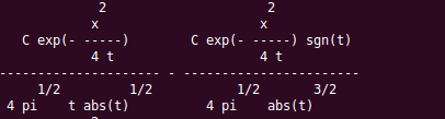
If we sample (I), we can see that it is all zero: symbolic solution is correct.
-
(S): ∂tf − i∂2xf:
d(f(x,t),t)-i*d(f(x,t),x,2)
fourier(last,x)
expand(last)
odesolve(last,fourier(f(x,t),x),t)
invfourier(last,x)
d(last,t)-i*d(last,x,2) (II)
We have the following symbolic solution:
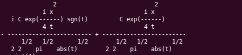
For (II) as for (I), the sample is all zero: symbolic solution is correct.
5.3 ↓Vectorial calculus
5.3.1 ↓↓Differential operators in↓ ↓orthogonal coordinate
We consider here orthogonal coordinates in
ℝ3 (i.e. a choice of three variables and a transformation). Using first form (cf. theory of surfaces) we define three operators (gradient of a scalar field
↓↓↓ ∇f, divergence of a vector field
↓↓↓ ∇.V, curl of a vector field
↓↓↓ ∇∧V, laplacian of a scalar field
↓↓↓ Δf, laplacian of a vector field
↓↓ ΔV = ∇(∇.V) − ∇∧(∇∧V)).
Then we test the following properties :
∇.(∇f) = Δf,
∇∧(∇f) = 0,
∇.(∇∧f) = 0.
The operators are constructed as follow :
-
gradient of a scalar field ∇f :
grado(f,Transf,Coord)=prog(FF,H,gradtemp,do(
FF=firstform(Transf,Coord),
H=(sqrt(FF[1,1]),sqrt(FF[2,2]),sqrt(FF[3,3])),
gradtemp=(1/H[1]*d(f,Coord[1]),1/H[2]*d(f,Coord[2]),1/H[3]*d(f,Coord[3])),
gradtemp))
-
divergence of a vector field ∇.V :
divo(V,Transf,Coord)=prog(FF,H,divtemp,do(
FF=firstform(Transf,Coord),
H=(sqrt(FF[1,1]),sqrt(FF[2,2]),sqrt(FF[3,3])),
divtemp=1/(H[1]*H[2]*H[3])*(d(V[1]*H[2]*H[3],Coord[1])+
d(V[2]*H[3]*H[1],Coord[2])+
d(V[3]*H[1]*H[2],Coord[3])),
divtemp))
-
curl of a vector field ∇∧V :
curlo(V,Transf,Coord)=prog(FF,H,curltemp,do(
FF=firstform(Transf,Coord),
H=(sqrt(FF[1,1]),sqrt(FF[2,2]),sqrt(FF[3,3])),
curltemp=(1/(H[2]*H[3])*(d(H[3]*V[3],Coord[2])-d(H[2]*V[2],Coord[3])),
1/(H[1]*H[3])*(d(H[1]*V[1],Coord[3])-d(H[3]*V[3],Coord[1])),
1/(H[1]*H[2])*(d(H[2]*V[2],Coord[1])-d(H[1]*V[1],Coord[2]))),
curltemp))
-
laplacian of a scalar field Δf :
laplo(f,Transf,Coord)=prog(FF,H,lapltemp,do(
FF=firstform(Transf,Coord),
H=(sqrt(FF[1,1]),sqrt(FF[2,2]),sqrt(FF[3,3])),
lapltemp=1/(H[1]*H[2]*H[3])*(d(H[2]*H[3]/H[1]*d(f,Coord[1]),Coord[1])+
d(H[3]*H[1]/H[2]*d(f,Coord[2]),Coord[2])+
d(H[1]*H[2]/H[3]*d(f,Coord[3]),Coord[3])),
lapltemp))
-
laplacian of a vector field ΔV :
vlaplo(V,Transf,Coord)=grado(divo(V,Transf,Coord),Transf,Coord)-
curlo(curlo(V,Transf,Coord),Transf,Coord)
In cartesian coordinates :
print()
print(Cartesian coordinates)
print()
Coord=(x,y,z)
Transf=(x,y,z)
V=(V1(),V2(),V3())
U=(U1(),U2(),U3())
print(div(grad)-lapl)
divo(grado(f(),Transf,Coord),Transf,Coord)-laplo(f(),Transf,Coord)
print(curl(grad))
curlo(grado(f(),Transf,Coord),Transf,Coord)
print(div(curl)) divo(curlo(V,Transf,Coord),Transf,Coord)
And smib gives :
Cartesian coordinates
div(grad)-lapl
0
curl(grad)
0
0
0
div(curl)
0
In cylindrical coordinates :
print()
print(Cylindrical coordinates)
print()
Coord=(r,phi,z)
Transf=(r*cos(phi),r*sin(phi),z)
V=(V1(),V2(),V3())
U=(U1(),U2(),U3())
print(div(grad)-lapl)
divo(grado(f(),Transf,Coord),Transf,Coord)-laplo(f(),Transf,Coord)
print(curl(grad))
curlo(grado(f(),Transf,Coord),Transf,Coord)
print(div(curl))
divo(curlo(V,Transf,Coord),Transf,Coord)
And smib gives :
Cylindrical coordinates
div(grad)-lapl
0
curl(grad)
0
0
0
div(curl)
0
5.3.2 ↓↓Vectorial integrals
Let
⟶a = (12cos(2t), − 8sin(2t), 16t) be
↓acceleration vector
↓, we want to compute speed vector
↓↓ ⟶v, position vector
↓↓ ⟶x.
In smib:
t=quote(t)
T=quote(T)
T1=quote(T1)
a=quote(a)
v=quote(v)
r=quote(r)
a=(12*cos(2*t),-8*sin(2*t),16*t)
v=defint(a,t,0,T)
r=defint(v,T,0,T1)
print("acceleration vector a=",a)
print("speed vector v=",v)
print("position vector r=",r)
And smib gives:
acceleration vector a= (12*cos(2*t),-8*sin(2*t),16*t)
speed vector v= (6*sin(2*T),-4+4*cos(2*T),8*T^2)
position vector r= (3-3*cos(2*T1),-4*T1+2*sin(2*T1),8/3*T1^3)
5.3.3 ↓↓Curvilinear integrals
-
Let C = {x(t) = 2t, t ∈ [0, 1]} a planar curve, andy(t) = 2t a function, we want to compute ∫Cy2ds. So in smib:
t=quote(t)
x=quote(x)
y=quote(y)
z=quote(z)
x=2t
y=2t
print("defint(y^2*d(x,t),t,0,1)=",defint(y^2*d(x,t),t,0,1))
And smib gives:
defint(y^2*d(x,t),t,0,1)= 8/3
-
Let C = {(x(t) = 2t + 1, y(t) = t2, z(t) = 1 + t3), t ∈ [0, 1]} a curve in ℝ3, and A⃗ = (z, x, y) a vector, we want to compute ∫CA⃗.ds. So in smib:
t=quote(t)
x=quote(x)
y=quote(y)
z=quote(z)
x=2t+1
y=t^2
z=1+t^3
f=z*d(x)+x*d(y)+y*d(z)
print("defint(z*d(x)+x*d(y)+y*d(z),t,0,1)=",defint(f,t,0,1))
And smib gives:
defint(z*d(x)+x*d(y)+y*d(z),t,0,1)= 163/30
-
Let C = {(x(t) = t2 + 1, y(t) = 2t2, z(t) = t3), t ∈ [1, 2]} a curve in ℝ3, and a vector F⃗ = (3xy, − 5z, 10x), we want to compute ∫CF⃗.ds. So in smib:
t=quote(t)
x=quote(x)
y=quote(y)
z=quote(z)
F=quote(F)
G=quote(G)
C=quote(C)
x=t^2+1
y=2*t^2
z=t^3
F=(3*x*y,-5*z,10*x)
C=(x,y,z)
print("defint(dotP(F,d(C,t)),t,1,2)=",defint(dotP(F,d(C,t)),t,1,2))
And smib gives:
defint(dotP(F,d(C,t)),t,1,2)= 303
-
Let C = {(x(t) = t2, y(t) = 2t, z(t) = t3), t ∈ [1, 2]} a curve in ℝ3,φ = 2xyz2 a function and F⃗ = (xy, − z, x2) a vector, we want to compute ∫Cφds and ∫CF⃗∧ds. So in smib:
t=quote(t)
x=quote(x)
y=quote(y)
z=quote(z)
F=quote(F)
phi=quote(phi)
G=quote(G)
C=quote(C)
x=t^2
y=2*t
z=t^3
phi=2*x*y*z^2
F=(x*y,-z,x^2)
C=(x,y,z)
print("defint(phi*d(C,t),t,0,1)=",defint(phi*d(C,t),t,0,1))
print("defint(crossP(F,d(C,t)),t,0,1)=",defint(crossP(F,d(C,t)),t,0,1))
And smib gives:
defint(phi*d(C,t),t,0,1)= (8/11,4/5,1)
defint(crossP(F,d(C,t)),t,0,1)= (-9/10,-2/3,7/5)
5.3.4 Area integrals↓↓
-
Let S = {(x, y, x2 + 2y), (x, y) ∈ [0, 1]2} a map in ℝ3, we want to compute ∬SdS. So in smib:
a=quote(a)
t=quote(t)
x=quote(x)
y=quote(y)
z=quote(z)
z=x^2+2y
S=(x,y,z)
a=abs(crossP(d(S,x),d(S,y)))
print("S=",S)
print("defint(defint(abs(crossP(d(S,x),d(S,y))),x,0,1),y,0,1)=",
defint(defint(a,x,0,1),y,0,1))
And smib gives:
S= (x,y,2*y+x^2)
defint(defint(abs(crossP(d(S,x),d(S,y))),x,0,1),y,0,1)=
1/2*(3-5/2*log(2)-5/4*log(5)+5/2*log(10))
-
Let S = {(ucos(v), usin(v), v), (u, v) ∈ [0, 1] × [0, 3π]} a map in ℝ3, we want to compute ∬SdS. So in smib:
a=quote(a)
t=quote(t)
u=quote(u)
v=quote(v)
x=quote(x)
y=quote(y)
z=quote(z)
x=u*cos(v)
y=u*sin(v)
z=v
S=(x,y,z)
a=abs(crossP(d(S,u),d(S,v)))
a=simplify(a)
print("S=",S)
print("defint(defint(abs(crossP(d(S,u),d(S,v))),u,0,1),v,0,3pi)=",
defint(defint(a,u,0,1),v,0,3pi))
And smib gives:
S= (u*cos(v),u*sin(v),v)
defint(defint(abs(crossP(d(S,u),d(S,v))),u,0,1),v,0,3pi)=
-3/2*pi*log(2)+3/2*pi*log(2+2*2^(1/2))+3*pi/(2^(1/2))
5.3.5 Some famous theorems
We want to test Green theorem: let C = {(cos(t), sin(t)), t ∈ [0, 2π]} a planar closed curve, S such that C = ∂S, S = {(rcos(t), rsin(t)), (r, t) ∈ [0, 1] × [0, 2π]}, P = 2x3 − y3, and Q = x3 + y3, now we want to verify: ∫CPdx + Qdy = ∬S(∂yP − ∂xQ)dS.
So in smib:
r=quote(r)
t=quote(t)
x=quote(x)
y=quote(y)
z=quote(z)
P=2x^3-y^3
Q=x^3+y^3
f=d(Q,x)-d(P,y)
x=r*cos(theta)
y=r*sin(theta)
f=expand(f)
print("integral(d(Q,x)-d(P,y))=",defint(defint(f*r,r,0,1),theta,0,2pi))
t=quote(t)
x=quote(x)
y=quote(y)
z=quote(z)
x=cos(t)
y=sin(t)
P=2x^3-y^3
Q=x^3+y^
f=expand(P*d(x,t)+Q*d(y,t))
print("integral(P*d(x,t)+Q*d(y,t))=",defint(f,t,0,2pi))
And smib gives:
integral(d(Q,x)-d(P,y))= 3/2*pi
integral(P*d(x,t)+Q*d(y,t))= 3/2*pi
We propose to evaluate Stokes theorem on two examples:
-
Let S a map in ℝ3defined by S = {(x, y, 4 − x2 − y2), (x, y) ∈ [ − 1, 1]2}, and ⟶F = (y, z, x)
-
Let S a map in ℝ3 defined by S = {(x, y, √(1 − x2 − y2)), (x, y) ∈ [ − 1, 1]2}, and ⟶F = (2x − y, − x2y, − y2z).
From these assumptions, we want to verify: ∫∂S⟶F.dr = ∬S⟶∇∧⟶F.dS.
So in smib:
Example 1:
print("Map integral")
t=quote(t)
x=quote(x)
y=quote(y)
z=quote(z)
X=(x,y,z)
Transf=(x,y,z)
z=4-x^2-y^2
F=(y,z,x)
S=(x,y,z)
f=expand(dot(curlo(F,Transf,X),crossP(d(S,x),d(S,y))))
x=r*cos(theta)
y=r*sin(theta)
f=simplify(f)
print("integral(dot(Rot(F,X),crossP(d(S,x),d(S,y))))=",
defint(defint(f*r,r,0,2),theta,0,2pi))
print("Curvilinear integral")
t=quote(t)
x=quote(x)
y=quote(y)
z=quote(z)
x=2*cos(t)
y=2*sin(t)
z=4-x^2-y^2
P=F[1]
Q=F[2]
R=F[3]
f=expand(P*d(x,t)+Q*d(y,t)+R*d(z,t))
print("integral(P*d(x,t)+Q*d(y,t)+R*d(z,t))=",defint(f,t,0,2pi))
print(" ")
And smib gives:
Map integral
integral(dot(Rot(F,X),crossP(d(S,x),d(S,y))))= -4*pi
Curvilinear integral
integral(P*d(x,t)+Q*d(y,t)+R*d(z,t))= -4*pi
Example 2:
t=quote(t)
x=quote(x)
y=quote(y)
z=quote(z)
phi=quote(phi)
theta=quote(theta)
X=(x,y,z)
Transf=(x,y,z)
F=(2*x-y,-x^2*y,-y^2*z)
print("Surface integral ")
z=sqrt(1-x^2-y^2)
S=(x,y,z)
f=expand(dot(curlo(F,Transf,X),
crossP(d(S,x),d(S,y))/sqrt(dot(crossP(d(S,x),d(S,y)),
crossP(d(S,x),d(S,y))))))
x=cos(phi)*cos(theta)
y=sin(phi)*cos(theta)
f=simplify(eval(f))
print("integral(dot(Rot(F,X),crossP(d(S,x),d(S,y))))=",
defint(defint(f*cos(theta),theta,0,pi/2),phi,0,2*pi))
print("Curvilinear integral")
t=quote(t)
x=quote(x)
y=quote(y)
z=quote(z)
x=cos(t)
y=sin(t)
z=sqrt(1-x^2-y^2)
P=F[1]
Q=F[2]
R=F[3]
f=expand(P*d(x,t)+Q*d(y,t)+R*d(z,t))
print("integral(P*d(x,t)+Q*d(y,t)+R*d(z,t))=",defint(f,t,0,2pi))
And smib gives:
Map integral
integral(dot(Rot(F,X),crossP(d(S,x),d(S,y))))= pi
Curvilinear integral
integral(P*d(x,t)+Q*d(y,t)+R*d(z,t))= pi
↓↓Gauss-Ostrogradski theorem
We will verify Gauss-Ostrogradski theorem: ∭V⟶∇.⟶FdV = ∬∂V⟶F.dS, for V = {(x = rcos(ϑ), y = rsin(ϑ), z), (r, ϑ, z) ∈ [0, 2] × [0, 2π] × [0, 3]}, and ⟶F = (4x, − 2y2, z2).
So in smib:
print("Volumic integral")
x=quote(x)
y=quote(y)
z=quote(z)
X=(x,y,z)
A=(4*x,-2*y^2,z^2)
print("Cylindrical coordinates")
r=quote(r)
theta=quote(theta)
z=quote(z)
Xcyl=(r,theta,z)
A1=subst(r*cos(theta),x,subst(r*sin(theta),y,A))
Coord=(r,theta,z)
Transf=(r*cos(theta),r*sin(theta),z)
M=((cos(theta),sin(theta),0),(-sin(theta),cos(theta),0),(0,0,1))
Acyl=dot(M,A1)
Bcyl=divo(simplify(Acyl),Transf,Xcyl)
Bcyl=simplify(Bcyl)
print("Bcyl = ",Bcyl)
print("integral(Div(A,X))=",defint(defint(defint(r*Bcyl,z,0,3),theta,0,2*pi),r,0,2))
print(" ")
print("Surfacic integral")
t=quote(t)
x=quote(x)
y=quote(y)
z=quote(z)
S1=(x,y,0)
print("S1: lower disk")
AS1=expand(dotP(A,crossP(d(S1,x),d(S1,y))))
x=r*cos(theta)
y=r*sin(theta)
z=0
IS1=defint(defint(expand(AS1*r),r,0,2),theta,0,2pi)
print("IS1=",IS1)
t=quote(t)
x=quote(x)
y=quote(y)
z=quote(z)
S2=(x,y,3)
print("S2: upper disk")
AS2=expand(dotP(A,crossP(d(S2,x),d(S2,y))))
x=r*cos(theta)
y=r*sin(theta)
z=3
IS2=defint(defint(expand(AS2*r),r,0,2),theta,0,2pi)
print("IS2=",IS2)
x=quote(x)
y=quote(y)
z=quote(z)
print("S3: cylindrical part")
S3=(x,sqrt(4-x^2),z)
AS3=dotP(A,crossP(d(S3,x),d(S3,z)))
x=r*cos(theta)
y=r*sin(theta)
r=2
z=quote(z)
IS3=defint(defint(simplify(expand(AS3*r)),theta,0,2pi),z,0,3)
print("IS3=",IS3)
print("IS1+IS2+IS3=",IS1+IS2+IS3)
And smib gives:
Volume integral
Cylindrical coordinates
Bcyl = 2*z-4*r*cos(theta)^2+4*r*sin(theta)^2-6*r*sin(theta)^3-
4*r^2*cos(theta)^2*sin(theta)+
2*r^2*sin(theta)^3+8*cos(theta)^2
integral(Div(A,X))= 84*pi
Surfacic integral
S1: lower disc
IS1= 0
S2: upper disc
IS2= 36*pi
S3: cylindrical part
IS3= 48*pi
5.4 Differential geometry↓
↓↓Planar curves
Here we want to study parametric planar curves
t:[a, b]⟼v⃗(t), we want to compute tangent vector
↓↓ T⃗ = v⃗̇⁄∥v⃗̇∥, normal vector
↓↓ N⃗ = ⎛⎜⎝
0
− 1
1
0
⎞⎟⎠T⃗, and curvature
↓ curR = ∥v⃗̇∥3⁄∥v⃗̇∧v⃗̈∥, so in smib:
curve2D(A,X)=prog(temp,temp1,temp2,
do(temp1=d(A,X),
temp2=d(temp1,X),
T=quote(T),T=simplify(temp1/normP(temp1)),
N=quote(N),N=inner(((0,-1),(1,0)),T),
curR=quote(curR),curR=simplify(normP(temp1)^3/cross2P(temp1,temp2))
Circle=(r*cos(t),r*sin(t))
print("Circle’s case:")
curve2D(Circle,t)
print("Tangent vector: T=",T)
print("Normal vector: N=",N)
print("Curvature: curR=",curR)
And the smib gives:
Circle’s case:
Tangent vector: T= (-sin(t),cos(t))
Normal vector: N= (-cos(t),-sin(t))
Curvature: curR= r
↓3D curves
And in 3D we have the following notions for a 3D parametric curve
t:[a, b]⟼v⃗(t), we want to compute: tangent vector
↓↓ T⃗ = v⃗̇⁄∥v⃗̇∥, normal vector
↓↓ N⃗ = T⃗̇⁄∥T⃗̇∥, binormal vector
↓↓ B⃗ = T⃗∧N⃗, curvature
↓ curR = ∥v⃗̇∥3⁄∥v⃗̇∧v⃗̈∥, and torsion
↓ curT = ∥v⃗̇∧v⃗̈∥⁄(v⃗̇∧v⃗̈).\overset...v⃗, so in smib:
curve3D(A,X)=prog(temp,temp1,temp2,temp3,
do(temp1=d(A,X),
temp2=d(temp1,X),
temp3=d(temp2,X),
T=quote(T),T=simplify(temp1/normP(temp1)),
temp=d(T,X),
N=quote(N),N=simplify(temp/normP(temp)),
B=quote(B),B=simplify(crossP(T,N)),
curR=quote(curR),
curR=simplify(normP(temp1)^3/normP(crossP(temp1,temp2))),
curT=quote(curT),
curT=-simplify(normP(crossP(temp1,temp2))/tripleSP(temp1,temp2,temp3))
))
And we apply this to ↓helix:
print("Helix case:")
h=quote(h)
r=quote(r)
Helix=(r*cos(t),r*sin(t),h*t)
curve3D(Helix,t)
print("Tangent vector: T=",T)
print("Normal vector: N=",N)
print("Binormal vector: B=",B)
print("Curvature: curR=",curR)
print("Torsion: curT=",curT)
And smib gives:
Helix case:
Tangent vector:
T= (r*sin(t)/((h^2+r^2)^(1/2)),r*cos(t)/((h^2+r^2)^(1/2)),h/((h^2+r^2)^(1/2)))
Normal vector: N= (cos(t),-sin(t),0)
Binormal vector:
B= (h*sin(t)/((h^2+r^2)^(1/2)),h*cos(t)/((h^2+r^2)^(1/2)),r/((h^2+r^2)^(1/2)))
Curvature: curR= r+h^2/r
Torsion: curT= -(h^2+r^2)^(1/2)/(h*r)
5.4.2 ↓Theory of surfaces
After curves, we are logically going to study surfaces, first we start with gaussian theory which is efficient with 2D surfaces, and after with riemannian theory which is efficient in all dimension.
Let S:(u, v)⟼(x1(u, v), x2(u, v), x3(u, v)) be a map discribing a 2D surface, we want to compute:
-
↓↓first form, and its determinant↓,
-
↓↓normal vector,
-
↓↓second form,
-
↓↓Weingarten operator,
-
↓↓Mean curvature, Gaussian curvature↓↓, and principal curvature↓↓,
-
↓Shape index↓ and curvedness↓.
So in smib:
gauss(A,X)=prog(temp1,temp2,temp11,temp12,temp22,
do(temp1=d(A,X[1]),
temp2=d(A,X[2]),
temp11=d(temp1,X[1]),
temp12=d(temp1,X[2]),
temp22=d(temp2,X[2]),
E=quote(E),E=simplify(dotP(temp1,temp1)),
F=quote(F),F=simplify(dotP(temp1,temp2)),
G=quote(G),G=simplify(dotP(temp2,temp2)),
I=quote(I),I=((E,F),(F,G)),
g=quote(g),g=simplify(det(I)),
h=quote(h),
h=simplify(simplify(crossP(temp1,temp2)/
sqrt(dotP(crossP(temp1,temp2),crossP(temp1,temp2))))),
h1=quote(h1),h1=simplify(d(h,X[1])),
h2=quote(h2),h2=simplify(d(h,X[2])),
L=quote(L),L=simplify(dotP(h,temp11)),
M=quote(M),M=simplify(dotP(h,temp12)),
N=quote(N),N=simplify(dotP(h,temp22)),
II=quote,II=simplify(((L,M),(M,N))),
b=quote(b),b=det(II),
W=quote(W),W=simplify(inner(II,inv(I))),
H=quote(H),H=simplify(contr(W,1,2)/2),
K=quote(K),K=simplify(det(W)),
chi1=quote(chi1),chi2=quote(chi2),
chi1=simplify(H+sqrt(H^2-K)),
chi2=simplify(H-sqrt(H^2-K)),
S=test(chi1==chi2,1,
2*(arctan(simplify((chi1+chi2)/(chi1-chi2))))/pi),
C=quote(C),C=2*(log(simplify(sqrt(chi1^2+chi2^2)/2)))/pi
))
We could test too ↓↓Gauss equations, Gauss theorem↓↓, Mainardi-Codazzi equations↓↓, and Bonnet theorem↓↓, those tests could be implemented as:
bonnet(E,F,G,L,M,N)=prog(temp1,temp2,
do(b=simplify(L*N-M^2),
g=simplify(E*G-F^2),
G111=simplify((d(E,X[1])*G-2*F*d(F,X[1])+d(E,X[2])*F)/(2*g)),
G211=simplify((-d(E,X[1])*F-2*E*d(F,X[1])+d(E,X[2])*E)/(2*g)),
G112=simplify((d(E,X[2])*G-F*d(G,X[1]))/(2*g)),
G121=G112,
G212=simplify((d(G,X[1])*E-F*d(E,X[2]))/(2*g)),
G221=G212,
G122=simplify(-(d(G,X[2])*F-2*F*d(G,X[2])+d(G,X[1])*G)/(2*g)),
G222=simplify((d(G,X[2])*E-2*F*d(F,X[2])+d(G,X[1])*F)/(2*g)),
temp1=simplify(F*b/g),
temp2=simplify(d(G112,X[1])-d(G111,X[2])+
G112*G212-G211*G122),
check(temp1-temp2),
print("Gauss 1st equation: ok"),
temp1=simplify(-E*b/g),
temp2=simplify(d(G212,X[1])-d(G211,X[2])+
G112*G211-G211*G222+ G212*(G212-G111)),
check(temp1-temp2),
print("Gauss 2nd equation: ok"),
temp1=simplify(G*b/g),
temp2=simplify(d(G122,X[1])-d(G112,X[2])+
G111*G122-G212*G122+G112*(G222-G112)),
check(temp1-temp2),
print("Gauss 3rd equation: ok"),
temp1=simplify(F*b/g),
temp2=simplify(d(G222,X[1])-d(G212,X[2])+G112*G211-G122*G211),
check(temp1-temp2),
print("Gauss 4th equation: ok"),
print("Gauss’s theorem:ok"),
temp1=simplify(d(L,X[2])-d(M,X[1])),
temp2=simplify(G112*L+(G212-G111)*M-G211*N),
check(temp1-temp2),
print("Mainardi-Codazzi 1st equation: ok"),
temp1=simplify(d(M,X[2])-d(N,X[1])),
temp2=simplify(G122*L+(G222-G112)*M-G212*N),
check(temp1-temp2),
print("Mainardi-Codazzi 2nd equation: ok"),
print("Bonnet’s theorem:ok")))
Now, we are going to test it on:
A ↓sphere:
Sphere case: (cos(v)*sin(u),sin(u)*sin(v),cos(u))
First form: I= ((1,0),(0,sin(u)^2))
Determinant of first form: g= sin(u)^2
Normal vector: h= (cos(v)*sin(u),sin(u)*sin(v),cos(u))
Second form: II= ((-1,0),(0,-sin(u)^2))
Weingarten’s operator: W= ((-1,0),(0,-1))
Mean curvature: H= -1
Gaussian curvature: K= 1
Principal curvatures:
chi1: -1
chi2: -1
Shape index: S= 1
Curvedness: C= -log(2)/pi
Gauss 1st equation: ok
Gauss 2nd equation: ok
Gauss 3rd equation: ok
Gauss 4th equation: ok
Gauss ’s theorem:ok
Mainardi-Codazzi 1st equation: ok
Mainardi-Codazzi 2nd equation: ok
Bonnet’s theorem:ok
A ↓cylinder:
Cylinder case: (sin(u),cos(u),v)
First form: I= ((1,0),(0,1))
Determinant of first form: g= 1
Normal vector: h= (-sin(u),-cos(u),0)
Second form: II= ((1,0),(0,0))
Weingarten’s operator: W= ((1,0),(0,0))
Mean curvature: H= 1/2
Gaussian curvature: K= 0
Principal curvatures:
chi1: 1
chi2: 0
Shape index: S= 1/2
Curvedness: C= -2*log(2)/pi
Gauss 1st equation: ok
Gauss 2nd equation: ok
Gauss 3rd equation: ok
Gauss 4th equation: ok
Gauss theorem: ok
Mainardi-Codazzi 1st equation: ok
Mainardi-Codazzi 2nd equation: ok
Bonnet theorem: ok
A ↓torus:
Torus case: (cos(u)+cos(u)*cos(v),cos(v)*sin(u)+sin(u),sin(v))
First form: I= ((1+2*cos(v)+cos(v)^2,0),(0,1))
Determinant of first form: g= 1+2*cos(v)+cos(v)^2
Normal vector: h= (cos(u)*cos(v),cos(v)*sin(u),sin(v))
Second form: II= ((-1-cos(v)+sin(v)^2,0),(0,-1))
Weingarten’s operator: W= ((-cos(v)/(1+2*cos(v)+cos(v)^2)+
sin(v)^2/(1+2*cos(v)+cos(v)^2)-1/(1+2*cos(v)+cos(v)^2),0),(0,-1))
Mean curvature: H= -1/2-cos(v)/(2+4*cos(v)+2*cos(v)^2)+
sin(v)^2/(2+4*cos(v)+2*cos(v)^2)-1/(2+4*cos(v)+2*cos(v)^2)
Gaussian curvature: K= cos(v)/(1+2*cos(v)+cos(v)^2)-sin(v)^2/(1+2*cos(v)+cos(v)^2)+
1/(1+2*cos(v)+cos(v)^2)
Principal curvature:
chi1: -1/2-cos(v)/(2+4*cos(v)+2*cos(v)^2)-cos(v)^2/(2+4*cos(v)+2*cos(v)^2)+
(1/4-cos(v)/(1+2*cos(v)+cos(v)^2)-cos(v)^2/(1+2*cos(v)+cos(v)^2)+
cos(v)^2/((2+4*cos(v)+2*cos(v)^2)^2)+2*cos(v)^3/((2+4*cos(v)+2*cos(v)^2)^2)+
cos(v)^4/((2+4*cos(v)+2*cos(v)^2)^2)+cos(v)/(2+4*cos(v)+2*cos(v)^2)+
cos(v)^2/(2+4*cos(v)+2*cos(v)^2))^(1/2)
chi2: -1+cos(v)/(2+4*cos(v)+2*cos(v)^2)-(1/4-cos(v)/(1+2*cos(v)+cos(v)^2)-
cos(v)^2/(1+2*cos(v)+cos(v)^2)+cos(v)^2/((2+4*cos(v)+2*cos(v)^2)^2)+
2*cos(v)^3/((2+4*cos(v)+2*cos(v)^2)^2)+cos(v)^4/((2+4*cos(v)+2*cos(v)^2)^2)+
cos(v)/(2+4*cos(v)+2*cos(v)^2)+cos(v)^2/(2+4*cos(v)+2*cos(v)^2))^(1/2)+
1/(2+4*cos(v)+2*cos(v)^2)
Shape index: S= 2*arctan(2*(-2-10*cos(v)-18*cos(v)^2-14*cos(v)^3-
4*cos(v)^4)/((1/2-2*cos(v)/(2+4*cos(v)+2*cos(v)^2)-
cos(v)^2/(2+4*cos(v)+2*cos(v)^2)+2*(1/4-cos(v)/(1+2*cos(v)+cos(v)^2)-
cos(v)^2/(1+2*cos(v)+cos(v)^2)+cos(v)^2/((2+4*cos(v)+2*cos(v)^2)^2)+
2*cos(v)^3/((2+4*cos(v)+2*cos(v)^2)^2)+cos(v)^4/((2+4*cos(v)+2*cos(v)^2)^2)+
cos(v)/(2+4*cos(v)+2*cos(v)^2)+cos(v)^2/(2+4*cos(v)+2*cos(v)^2))^(1/2)-
1/(2+4*cos(v)+2*cos(v)^2))*(2+4*cos(v)+2*cos(v)^2)^2))/pi
Curvedness: C= -2*log(2)/pi+log(7/4-2*(1/4-cos(v)/(1+2*cos(v)+cos(v)^2)-
cos(v)^2/(1+2*cos(v)+cos(v)^2)+cos(v)^2/((2+4*cos(v)+2*cos(v)^2)^2)+
2*cos(v)^3/((2+4*cos(v)+2*cos(v)^2)^2)+cos(v)^4/((2+4*cos(v)+
2*cos(v)^2)^2)+cos(v)/(2+4*cos(v)+2*cos(v)^2)+
cos(v)^2/(2+4*cos(v)+2*cos(v)^2))^(1/2)/(2+4*cos(v)+2*cos(v)^2)-
4*(1/4-cos(v)/(1+2*cos(v)+cos(v)^2)-cos(v)^2/(1+2*cos(v)+cos(v)^2)+
cos(v)^2/((2+4*cos(v)+2*cos(v)^2)^2)+2*cos(v)^3/((2+4*cos(v)+2*cos(v)^2)^2+
cos(v)^4/((2+4*cos(v)+2*cos(v)^2)^2)+cos(v)/(2+4*cos(v)+2*cos(v)^2)+
cos(v)^2/(2+4*cos(v)+2*cos(v)^2))^(1/2)*cos(v)/(2+4*cos(v)+2*cos(v)^2)-
2*(1/4-cos(v)/(1+2*cos(v)+cos(v)^2)-cos(v)^2/(1+2*cos(v)+cos(v)^2)+
cos(v)^2/((2+4*cos(v)+2*cos(v)^2)^2)+2*cos(v)^3/((2+4*cos(v)+
2*cos(v)^2)^2)+cos(v)^4/((2+4*cos(v)+2*cos(v)^2)^2)+
cos(v)/(2+4*cos(v)+2*cos(v)^2)+cos(v)^2/(2+4*cos(v)+
2*cos(v)^2))^(1/2)*cos(v)^2/(2+4*cos(v)+2*cos(v)^2)-
2*cos(v)/(1+2*cos(v)+cos(v)^2)-2*cos(v)^2/(1+2*cos(v)+cos(v)^2)+
2*cos(v)/((2+4*cos(v)+2*cos(v)^2)^2)+4*cos(v)^2/((2+4*cos(v)+2*cos(v)^2)^2)
+6*cos(v)^3/((2+4*cos(v)+2*cos(v)^2)^2)+
3*cos(v)^4/((2+4*cos(v)+2*cos(v)^2)^2)+cos(v)/(2+4*cos(v)+2*cos(v)^2)+
3*cos(v)^2/(2+4*cos(v)+2*cos(v)^2)+(1/4-cos(v)/(1+2*cos(v)+cos(v)^2)-
cos(v)^2/(1+2*cos(v)+cos(v)^2)+cos(v)^2/((2+4*cos(v)+2*cos(v)^2)^2)+
2*cos(v)^3/((2+4*cos(v)+2*cos(v)^2)^2)+cos(v)^4/((2+4*cos(v)+2*cos(v)^2)^2)+
cos(v)/(2+4*cos(v)+2*cos(v)^2)+cos(v)^2/(2+4*cos(v)+2*cos(v)^2))^(1/2)+
(2+4*cos(v)+2*cos(v)^2)^(-2)-2/(2+4*cos(v)+2*cos(v)^2))/pi
As we could see simplification felt out for torus... Another smib weakness↓!
5.4.3 ↓Riemannian geometry
Instead of using a parametric representation of a surface, we use notion of metric
↓. Hereafter are some examples in several dimensions, we compute
↓↓connection coefficient( or
↓↓Christoffel symbol), Riemann tensor
↓↓, Ricci tensor
↓↓, Ricci curvature
↓↓ , and Laplace operator
↓.
-
↓↓Nil: ds2 = dx2 + dy2 + ( − xdy + dz)2
X=(x,y,z) print("Nil")
A=((1,0,0),(0,1+x^2,-x),(0,-x,1))
riemann(A,X)
print("Metric: gdd=",gdd)
print("Connection: GAMUDD=",GAMUDD)
print("Riemann tensor RUDDD=",RUDDD)
print("Ricci tensor RDD=",RDD)
print("Ricci Curvature R=",R)
f=quote(f)
print("LaplF(f(X),X)=",LaplF(f(X),X))
print(" ")
And smib gives:
Metric: gdd= ((1,0,0),(0,1+x^2,-x),(0,-x,1))
Connection: GAMUDD=
(((0,0,0),(0,-x,1/2),(0,1/2,0)),
((0,1/2*x,-1/2),(1/2*x,0,0),(-1/2,0,0)),
((0,-1/2+1/2*x^2,-1/2*x),(-1/2+1/2*x^2,0,0),(-1/2*x,0,0)))
Riemann tensor RUDDD=
((((0,0,0),(0,0,0),(0,0,0)),
((0,-3/4+1/4*x^2,-1/4*x),(3/4-1/4*x^2,0,0),(1/4*x,0,0)),
((0,-1/4*x,1/4),(1/4*x,0,0),(-1/4,0,0))),
(((0,3/4,0),(-3/4,0,0),(0,0,0)),
((0,0,0),(0,0,-1/4*x),(0,1/4*x,0)),
((0,0,0),(0,0,1/4),(0,-1/4,0))),
(((0,x,-1/4),(-x,0,0),(1/4,0,0)),
((0,0,0),(0,0,-1/4-1/4*x^2),(0,1/4+1/4*x^2,0)),
((0,0,0),(0,0,1/4*x),(0,-1/4*x,0))))
Ricci tensor RDD=
((-1/2,0,0),(0,-1/2+1/2*x^2,-1/2*x),(0,-1/2*x,1/2))
Ricci Curvature R= -1/2
LaplF(f(X),X)=
d(d(f((x,y,z)),x),x)+d(d(f((x,y,z)),y),y)+d(d(f((x,y,z)),z),z)+
2*x*d(d(f((x,y,z)),y),z)+x^2*d(d(f((x,y,z)),z),z)
-
Sol↓↓: ds2 = e2xds2 + e − 2xdy2 + dz2
X=(x,y,z)
print("Sol")
A=((exp(2*x),0,0),(0,exp(-2*x),0),(0,0,1))
riemann(A,X)
print("Metric: gdd=",gdd)
print("Connection: GAMUDD=",GAMUDD)
print("Riemann tensor RUDDD=",RUDDD)
print("Ricci tensor RDD=",RDD)
print("Ricci Curvature R=",R)
f=quote(f)
print("LaplF(f(X),X)=",LaplF(f(X),X))
And smib gives:
Sol Metric: gdd= ((exp(2*x),0,0),(0,exp(-2*x),0),(0,0,1))
Connection: GAMUDD=(((1,0,0),(0,exp(-4*x),0),(0,0,0)),
((0,-1,0),(-1,0,0),(0,0,0)),
((0,0,0),(0,0,0),(0,0,0)))
Riemann tensor RUDDD=
((((0,0,0),(0,0,0),(0,0,0)),
((0,-2*exp(-4*x),0),(2*exp(-4*x),0,0),(0,0,0)),
((0,0,0),(0,0,0),(0,0,0))),
(((0,2,0),(-2,0,0),(0,0,0)),
((0,0,0),(0,0,0),(0,0,0)),
((0,0,0),(0,0,0),(0,0,0))),
(((0,0,0),(0,0,0),(0,0,0)),
((0,0,0),(0,0,0),(0,0,0)),
((0,0,0),(0,0,0),(0,0,0))))
Ricci tensor RDD= ((-2,0,0),(0,-2*exp(-4*x),0),(0,0,0))
Ricci Curvature R= -4*exp(-2*x)
LaplF(f(X),X)= d(d(f((x,y,z)),z),z)+exp(-2*x)*d(d(f((x,y,z)),x),x)
-2*exp(-2*x)*d(f((x,y,z)),x)+exp(2*x)*d(d(f((x,y,z)),y),y)
-
↓↓Schwarzschild metric:
X=(x1,x2,x3,x4) gdd=((-x1/(x1-a),0,0,0),(0,-x1^2,0,0),
(0,0,-x1^2*sin(x2)^2,0),(0,0,0,-(x1-a)/x1))
print("gdd=",gdd)
riemann(gdd,X)
print("GAMUDD[2,1,2]=",simplify(GAMUDD[2,1,2]))
print("GAMUDD[3,1,3]=",simplify(GAMUDD[3,1,3]))
print("RDD=",simplify(RDD))
print("R=",simplify(R))
smib gives:
gdd= ((-x1/(-a+x1),0,0,0),(0,-x1^2,0,0),
(0,0,-x1^2*sin(x2)^2,0),(0,0,0,-1+a/x1))
GAMUDD[2,1,2]= 1/x1
GAMUDD[3,1,3]= 1/x1
RDD= 0
R= 0
-
The following function allows the testing of some properties of tensors and covariant derivative↓↓.
testgdd()=prog(tmp,tmp1,tmp2,tmp3,do(
print("Commutator is anticommutative:"),
test(Commutator(V,W)+Commutator(W,V)==0,
print("Commutator(V,W)+Commutator(W,V)==0: ok"),
print("Commutator(V,W)+Commutator(W,V)==0: ko")), print("Commutator is linear: 1 "),
test(Commutator(V+U,W)-(Commutator(V,W)+Commutator(U,W))==0,
print("Commutator(V+U,W)-(Commutator(V,W)+Commutator(U,W))==0: ok"),
print("Commutator(V+U,W)-(Commutator(V,W)+Commutator(U,W))==0: ko")),
print("Commutator is linear: 2 "),
test(Commutator(V,W+U)-(Commutator(V,W)+Commutator(V,U))==0,
print("Commutator(V,W+U)-(Commutator(V,W)+Commutator(V,U))==0: ok"),
print("Commutator(V,W+U)-(Commutator(V,W)+Commutator(V,U))==0: ko")),
print("Jacobi identity:"),
test(Commutator(Commutator(U,V),W)+Commutator(Commutator(V,W),U)+Commutator(Commutator(W,U),V)==0,
print("Commutator(Commutator(U,V),W)+Commutator(Commutator(V,W),U)+Commutator(Commutator(W,U),V)==0: ok"),
print("Commutator(Commutator(U,V),W)+Commutator(Commutator(V,W),U)+Commutator(Commutator(W,U),V)==0:ko")),
print("Symmetry of covariant derivative: "),
test(DirCovDerVU(V,W)-DirCovDerVU(W,V)-Commutator(W,V)==0,
print("DirCovDerVU(V,W)-DirCovDerVU(W,V)-Commutator(W,V)==0: ok"),
print("DirCovDerVU(V,W)-DirCovDerVU(W,V)-Commutator(W,V)==0: ko")),
print("Composition rule: " ),
test(DirCovDerVU(f(X)*V,W)-f(X)*DirCovDerVU(V,W)-outer(V,contr(outer(d(f(X),X),W),1,2))==0,
print("DirCovDerVU(f(X)*V,W)-f(X)*DirCovDerVU(V,W)-outer(V,contr(outer(d(f(X),X),W),1,2))==0: ok"),
print("DirCovDerVU(f(X)*V,W)-f(X)*DirCovDerVU(V,W)-outer(V,contr(outer(d(f(X),X),W),1,2))==0: ko")),
print("Additivity of covariant derivative: "),
test(DirCovDerVU(U,V+W)-DirCovDerVU(U,V)-DirCovDerVU(U,W)==0,
print("DirCovDerVU(U,V+W)-DirCovDerVU(U,V)-DirCovDerVU(U,W)==0: ok"),
print("DirCovDerVU(U,V+W)-DirCovDerVU(U,V)-DirCovDerVU(U,W)==0: ko")),
test(RUDDD-(1/2*(RUDDD-trans(RUDDD,3,4)))==0,
print("Riemann tensor is antisymmetric on two last indices: ok"),
print("Riemann tensor is antisymmetric on two last indices: ko")), test(contr(outer(guu,RDDDD),2,3)==0,
print("Is metric flat?: Yes"),
print("Is metric flat?: No")),
test(CovDerTUD(CovDerVU(V,X),X)-trans(CovDerTUD(CovDerVU(V,X),X),2,3)-trans(contr(outer(RUDDD,V),2,5),2,3)==0,
print("Covariant derivative is not flat: ok"),
print("Covariant derivative is not flat: ko")),
test(simplify(CovDerTDD(gdd,X))==0,
print("CovDerTDD(gdd,X)=0: ok"),
print("CovDerTDD(gdd,X)=0: ko")),
test(contr(CovDerTUU(GUU,X),2,3)==0,
print("Div(GUU)=0: ok"),
print("Div(GUU)=0: ko")),
print("testgdd: ok")
) )
Now we can apply this to ↓↓statical-spherical metric, with this script:
a=quote(a)
b=quote(b)
X4=(x0,x1,x2,x3)
W4=(w0(X4),w1(X4),w2(X4),w3(X4))
V4=(v0(X4),v1(X4),v2(X4),v3(X4))
U4=(u0(X4),u1(X4),u2(X4),u3(X4))
V=V4
U=U4
W=W4
X=X4
Staticspherical = ((a(x0,x1), 0, 0, 0), (0, b(x0,x1), 0, 0),
(0, 0, x1^2, 0), (0, 0, 0, x1^2 sin(x2)^2))
riemann(Staticspherical,X)
print("Metric: gdd=",gdd)
testgdd()
And smib gives:
5.5 ↓Numerical analysis
5.5.1 Sample↓s applied to numerical analysis
Here we want to study the function f:x⟼exp( − x2) using samples. We will look at the following properties:
- first and second order derivative of f (comparison of samples with symbolic computations)
- test if
f verifies this
↓differential equation:
df⁄dx − xf = 0
- test if ∫df⁄dxdx = f (fundamental theorem of analysis).
Here, we choose sampling interval I = [ − 3, 3], and sampling rate N = 200, and here, we measure the error with the function Snorm.
So in smib:
N=200
a=3
f=exp(-x^2)
print("f= ",f)
A=sample(f,x,-a,a,N)
X=sample(x,x,-a,a,N)
SDf=Sd(A)
Df=sample(d(f,x),x,-a,a,N)
print("")
print("First order derivative")
print(Snorm(Sdiff(SDf,Df)))
SD2f=Sd(SDf)
D2f=sample(d(f,x,2),x,-a,a,N)
print("")
print("Second order derivative")
print(Snorm(Sdiff(SD2f,D2f)))
print("")
print("Differential equation:d(f)+2xf=0")
print(Snorm(Ssum(SDf,Sscalarproduct(2,Sproduct(X,A)))))
print("")
print("Fundamental theorem of analysis")
g(x)=Sdefint(SDf,-a,x)
Z=sample(g,x,-a,a,N)
print(Snorm(Sdiff(A,Z)))
And smib gives:
f= exp(-x^2)
First order derivative
(0.00375495,0.000188644,0.000185906)
Second order derivative
(0.0200501,0.00101163,0.000988244)
Differential equation:d(f)+2xf=0
(0.00375495,0.000188644,0.000185906)
Fundamental theorem of analysis
(0.102201,0.0049872,0.0052051)
Here we plot ∫df⁄dxdx and f:
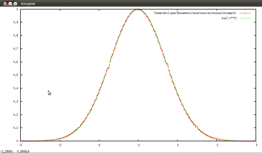
On the same principle, with
f:x⟼sin(x),
I = [ − 6, 6], and
N = 200, we have:
f= sin(x)
First order derivative
(0.0139451,0.00045642,0.000871306)
Second order derivative
(0.186432,0.00258752,0.0128928)
Fundamental theorem of analysis
(0.309026,0.018506,0.0115169)
Here we must be vigilant because sin( − 6) ≠ 0, so for fundamental theorem, we have the following code:
print("Fundamental theorem of analysis")
g(x)=Sdefint(SDf,-a,x)+sin(-6)
Z=sample(g,x,-a,a,N)
print(Snorm(Sdiff(A,Z)))
And the following plotting:

Here differential equation is
d²f⁄dx² + f = 0, so in smib:
print("Differential equation:d^2(f)+f=0")
print(Snorm(Ssum(SD2f,A)))
Result is:
Differential equation:d^2(f)+f=0
(0.186432,0.00258752,0.0128928)
If we plot error:
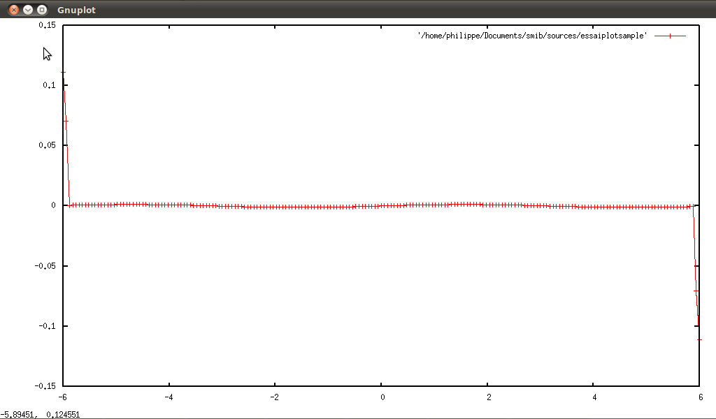
As we shall also see in paragraph on probability and statistics (
cf. quantile
↓ and median
↓), we can look at the following problem using the sample: let
F defined as
F(x) = ∫xaf(x)dx,
x ∈ [a, b], the problem is to find
x such that
F(x) = X.
We can also calculate the quantile
↓↓↓↓ (and median) of a sample with the following programs:
Squantile(f,a,b,y,errprec)=prog(temp0,temp1,temp2,
temp3,temp4,temp5,temp6,temp7,do(
test(b==nil,temp0=f[1,1],temp0=b),
test(y==nil,temp6=f[dim(f),1],temp6=y),
test(errprec==nil,temp7=0,temp7=errprec),
temp1=Sdefint(f,f[1,1],temp0)-a,
temp2=Sdefint(f,f[1,1],(temp0+temp6)/2)-a,
temp3=Sdefint(f,f[1,1],temp6)-a,
temp4=temp1*temp2,
temp5=temp2*temp3,
test(abs(abs(temp2)-temp7)==0,(temp0+temp6)/2,
test(and(temp4 < 0,temp5 > 0),
Squantile(f,a,(temp0+temp6)/2,temp0,temp6,abs(temp2)),
Squantile(f,a,(temp0+temp6)/2,temp6,abs(temp2))
)
)
))
And
Smedian(f)=Squantile(f,1/2)
We can test it on different function samples:
a=-5
b=5
N=1000
y0=30
f=x^2
print("f = ",f,", a = ",a,", b = ",b)
S=sample(f,x,a,b,N)
A=Squantile(S,y0)
I=Sdefint(S,a,A)
print("y0 = ",y0)
print("quantile = ",A)
print("check = ",I)
print("error = ",abs(y0-I))
And smib gives:
f = x^2 , a = -5 , b = 5
y0 = 30
quantile = -3.27
check = 29.94
error = 0.0599893
a=-5
b=5
N=1000
y0=50
f=x^2
print("f = ",f,", a = ",a,", b = ",b)
S=sample(f,x,a,b,N)
A=Squantile(S,y0)
I=Sdefint(S,a,A)
print("y0 = ",y0)
print("quantile = ",A)
print("check = ",I)
print("error = ",abs(y0-I))
And smib gives:
f = x^2 , a = -5 , b = 5
y0 = 50
quantile = 2.93457
check = 50.1086
error = 0.108583
a=-5
b=5
N=1000
y0=1/2
f=exp(-x^2)
print("f = ",f,", a = ",a,", b = ",b)
S=sample(f,x,a,b,N)
A=Squantile(S,y0)
I=Sdefint(S,a,A)
print("y0 = ",y0)
print("quantile = ",A)
print("check = ",I)
print("error = ",abs(y0-I))
And smib gives:
f = exp(-x^2) , a = -5 , b = 5
y0 = 1/2
quantile = -0.407715
check = 0.503734
error = 0.00373361
a=0.01
b=10
N=1000
y0=10
f=x*log(x)
print("f = ",f,", a = ",a,", b = ",b)
S=sample(f,x,a,b,N)
A=Squantile(S,y0)
I=Sdefint(S,a,A)
print("y0 = ",y0)
print("quantile = ",A)
print("check = ",I)
print("error = ",abs(num(y0-I)))
And smib gives:
f = x*log(x) , a = 0.01 , b = 10
y0 = 10
quantile = 4.47544
check = 9.95704
error = 0.042961
5.5.2 Special functions
Here we must be prudent, we must choose x such that |x| ≤ 10.
↓↓↓Bessel function of first kind:
J(x, α)
we choose the following definition:
J(x, α) = ∞⎲⎳j = 0( − 1)k(x⁄2)2j + α⁄j!Γ(α + j + 1)
So in smib:
numJ(x,p)=num(sum(k,0,prec,(-1)^k*(x/2)^(2*k+p)/(k!*Gamma(p+k+1))))
↓↓Bessel function of second kind:
Y(x, α)
we choose the following definition:
Y(x, α) = J(x, α)cos(απ) − J(x, − α)⁄sin(απ)
So in smib:
numY(x,p)=num((numJ(x,p)*cos(p*pi)-numJ(x,-p))/sin(p*pi))
↓↓↓Bessel modified function of first kind:
I(x, α)
we choose the following definition:
I(x, α) = i − αJ(ix, α)
So in smib:
numJ(x,p)=num(sum(k,0,prec,(-1)^k*(x/2)^(2*k+p)/(k!*Gamma(p+k+1))))
↓↓↓Hankel function of first kind:
H1(x, α)
we choose the following definition:
H1(x, α) = J(x, α) + iY(x, α)
So in smib:
numH1(x,p)=num(numJ(x,p)+i*numY(x,p))
↓↓Hankel function of second kind:
H2(x, α)
we choose the following definition:
H2(x, α) = J(x, α) − iY(x, α)
So in smib:
numH2(x,p)=num(numJ(x,p)-i*numY(x,p))
↓↓Bessel modified function of second kind:
K(x, α)
we choose the following definition:
K(x, α) = π⁄2iα + 1H1(ix, α)
So in smib:
numK(x,p)=num(pi/2*i^(p+1)*numH1(i*x,p))
↓↓Airy functions:
Ai(x, α) &
Bi(x, α)
we choose the following definitions:
Ai(x, α) = {
1⁄π√(x⁄3)K(2⁄3x3⁄2, 1⁄3), x > 0√( − x⁄3)(J(2⁄3( − x)3⁄2, 1⁄3) + J(2⁄3( − x)3⁄2, − 1⁄3))
Bi(x, α) = {
√( − x⁄3)(I(2⁄3( − x)3⁄2, 1⁄3) + I(2⁄3( − x)3⁄2, − 1⁄3)), x > 0√( − x⁄3)(J(2⁄3( − x)3⁄2, − 1⁄3) − J(2⁄3( − x)3⁄2, − 1⁄3))
So in smib:
numAi(x)=test(x>0,num(1/pi*sqrt(x/3)*numK(2*x^(3/2)/3,1/3)),
num(sqrt(-x)/3*(numJ(2*(-x)^(3/2)/3,1/3)+numJ(2*(-x)^(3/2)/3,-1/3))))
numBi(x)=test(x>0,num(sqrt(x/3)*(numI(2*x^(3/2)/3,1/3)+numI(2*x^(3/2)/3,-1/3))),
num(sqrt(-x/3)*(numJ(2*(-x)^(3/2)/3,-1/3)-numJ(2*(-x)^(3/2)/3,1/3))))
First some plottings:
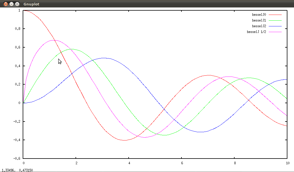
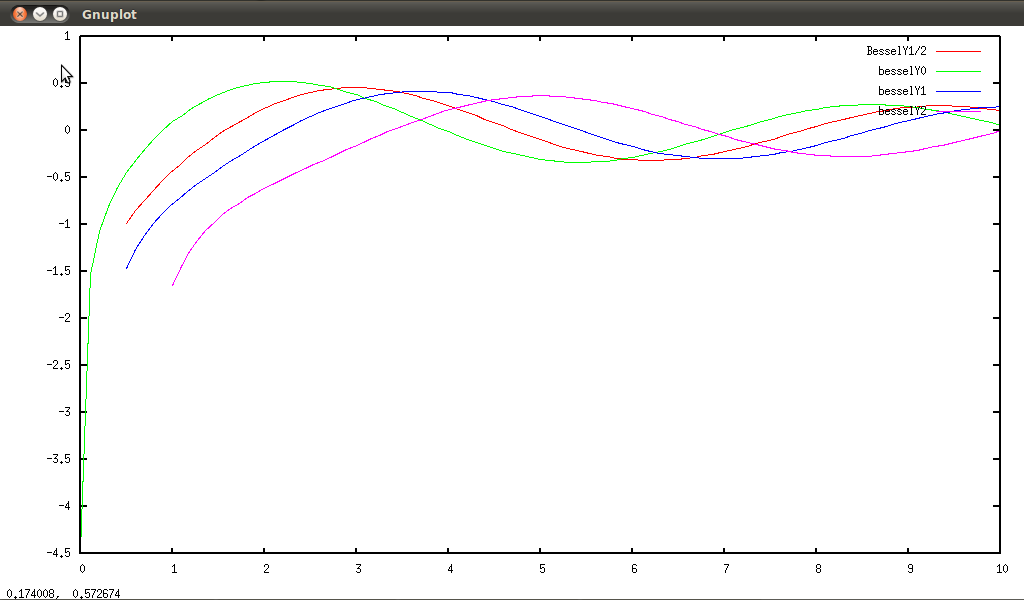
And after, some value computations:
numJ(2.5,0)= -0.0483838
numJ(2.5,2)= 0.446059
numJ(-2.5,0)= -0.0483838
numJ(-2.5,2)= 0.446059
numJ(2.5,1/2)= 0.302005
numJ(-2.5,1/2)= 0.302005*i
numY(2.5,1/2)= 0.404278
numY(-2.5,1/2)= -0.404278*i
numY(2.5,3/2)= -0.140294
numY(-2.5,3/2)= -0.140294*i
numN(2.5,1/2)= 0.404278
numN(-2.5,1/2)= -0.404278*i
numN(2.5,3/2)= -0.140294
numN(-2.5,3/2)= -0.140294*i
numH1(2.5,1/2)= 0.302005+0.404278*i
numH1(-2.5,1/2)= 0.404278+0.302005*i
numH1(2.5,3/2)= 0.52508-0.140294*i
numH1(-2.5,3/2)= 0.140294-0.52508*i
numH2(2.5,1/2)= 0.302005-0.404278*i
numH2(-2.5,1/2)= -0.404278+0.302005*i
numH2(2.5,3/2)= 0.52508+0.140294*i
numH2(-2.5,3/2)= -0.140294-0.52508*i
numI(2.5,0)= 3.28984
numI(-2.5,0)= 3.28984
numI(2.5,1/2)= 3.05309-6.66134e-16*i
numI(-2.5,1/2)= 6.66134e-16+3.05309*i
numK(2.5,1/2)= 0.0650659-6.93889e-18*i
numK(-2.5,1/2)= -2.66454e-15-9.65664*i
numK(2.5,3/2)= 0.0910923+2.42861e-16*i
numK(-2.5,3/2)= -1.33227e-15-5.79399*i
numAi(0.25)= 0.291164
numAi(1)= 0.135292+1.12218e-16*i
numAi(-0.25)= 0.418725
numAi(-1)= 0.535561
numBi(1)= 1.20742-6.40988e-17*i
numBi(-0.25)= 0.5014
numBi(-1)= 0.103997
The following examples introduce the section on numerical integration, indeed we are going to study the following integrals:
⎧⎪⎪⎪⎨⎪⎪⎪⎩
∫π⁄20J(2zsin(t), n)dt = π⁄2J(z, n⁄2)2
∫π0J(2zsin(t), 0)cos(2nt)dt = πJ(z, n)2
∫π⁄20Y(2zsin(t), 0)cos(2nt)dt = π⁄2J(z, n)Y(z, n)
∫z0J(t, n)J(z − t, − n)dt = sin(z)
∫z0J(t, n)J(z − t, 1 − n)dt = J(z, 0) − cos(z)
And smib gives:
I1(z,n)=numint(numJ(2*z*sin(t),n),t,0,pi/2)-pi/2*numJ(z,n/2)^2
I1(0.5,3)= -4.24834e-15
I1(2,3)= -2.70561e-13
I1(0.5,4)= -6.50521e-19
I1(2,4)= 1.11022e-16
I2(z,n)=numint(numJ(2*z*sin(t),0)*cos(2*n*t),t,0,pi)-pi*numJ(z,n)^2
I2(0.5,3)= -1.69302e-16
I2(2,3)= -1.45717e-16
I2(0.5,4)= -4.68064e-17
I2(2,4)= -1.01048e-16
I3(z,n)=numint(numY(2*z*sin(t),0)*cos(2*n*t),t,0,pi/2)-pi/2*numJ(z,n)*numY(z,n)
I3(0.5,1)= 0.0364192
I3(0.5,2)= 0.0364128
I3(2,1)= 0.0275907
I3(2,2)= 0.027586
I4(z,n)=numint(numJ(t,n)*numJ(z-t,-n),t,0,z)-sin(z)
I4(0,1/2)= 0.00636606*i
I4(0.5,1/2)= Stop: divide by zero
I4(0,1/3)= -0.00413489+0.00716184*i
I4(0.5,1/3)= Stop: divide by zero
I5(z,n)=numint(numJ(t,n)*numJ(z-t,1-n),t,0,z)-(numJ(z,0)-cos(z))
I5(0,1/2)= 0.00636606*i
I5(0.5,1/2)= Stop: divide by zero
I5(0,1/3)= 0
I5(0.5,1/3)= -2.10643e-06
I5(1,1/3)= -7.49049e-06
I5(2,1/3)= -1.74867e-05
As we could see that result are not always good (↓↓Simpson scheme), now we make the same exercise using Gauss scheme↓↓: simpsonint=0.
Then smib returns:
I1(z,n)=numint(numJ(2*z*sin(t),n),t,0,pi/2)-pi/2*numJ(z,n/2)^2
I1(0.5,3)= 6.33551e-05
I1(2,3)= 0.00139332
I1(0.5,4)= 8.01996e-06
I1(2,4)= 0.00091048
I2(z,n)=numint(numJ(2*z*sin(t),0)*cos(2*n*t),t,0,pi/2)-pi*numJ(z,n/2)^2
I2(0.5,3)= 0.0125691
I2(2,3)= 0.0157853
I2(0.5,4)= 0.0145211
I2(2,4)= -0.0306763
I3(z,n)=numint(numY(2*z*sin(t),0)*cos(2*n*t),t,0,pi/2)-pi/2*numJ(z,n)*numY(z,n)
I3(0.5,1)= 0.0253421
I3(0.5,2)= 0.0259082
I3(2,1)= 0.0196943
I3(2,2)= 0.0195847
I4(z,n)=numint(numJ(t,n)*numJ(z-t,-n),t,0,z)-sin(z)
I4(0,1/2)= 0.00639231*i
I4(0.5,1/2)= -0.000461072
I4(1,1/2)= -0.000178817
I4(2,1/2)= 7.98167e-05
I4(0,1/3)= -0.00415194+0.00719137*i
I4(0.5,1/3)= 0.00243214
I4(1,1/3)= 0.00587959
I4(2,1/3)= 0.00636122
I5(z,n)=numint(numJ(t,n)*numJ(z-t,1-n),t,0,z)+cos(z)-numJ(z,0)
I5(0,1/2)= 0.00639231*i
I5(0.5,1/2)= -0.000461072
I5(1,1/2)= -0.000178817
I5(2,1/2)= 7.98167e-05
I5(0,1/3)= 0
I5(0.5,1/3)= 1.78261e-05
I5(1,1/3)= 6.37467e-05
I5(2,1/3)= 0.000153571
And using Bessel function of second kind: I(z, n) = ∫z0J(t, n)J(z − t, − n)dt with qgfe, we obtain:
5.5.3 Numerical interpolation
Here we want to study Lagrange interpolation
↓ problem
↓ applied to a sample
F = (xi, yi)i ∈ {0..k}, we shall use Newton basis polynomials
↓ and
↓divide differences.
Newton polynomial is defined by:
Nj(x)=
∏i = j − 1i = 0(x − xi); and interpolation is implemanted (using temporary program)
↓ as:
newtonpoly(x,F,j)=product(ind,1,j,x-F[ind,1])
newtoninter(F,x)=prog(temp0,temp1,temp2,temp3,temp4,do(
temp1=Sdecomp(F,2),
temp4(F)=prog(temp,do(
temp=zero(dim(F),dim(F)),
for(ind1,1,dim(F),
for(ind2,1,dim(F),temp[ind1,ind2]=
newtonpoly(F[ind1,1],F,ind2-1)
)
),
return(temp)
)),
temp2=dot(inv(temp4(F)),temp1),
temp3=sum(ind,1,dim(F),temp2[ind]*newtonpoly(x,F,ind-1)),
return(temp3)
))
Hereafter two small examples:
a=-1.5
b=1.5
n=4
f=tan(x)
F=sample(f,x,a,b,n)
g=newtoninter(F,x)
G=sample(g,x,a,b,n)
Err=Sabs(Sdiff(F,G))
Snorm(Err)
And smib gives:
6.64652e-15
2.13163e-15
2.07157e-15
a=-5
b=5
n=20
f=x^2+1
F=sample(f,x,a,b,n)
g=newtoninter(F,x)
G=sample(g,x,a,b,n)
Err=Sabs(Sdiff(F,G))
Snorm(Err)
And smib gives:
5.69016e-08
5.17097e-09
1.1289e-08
Lagrange interpolation is interesting, but we can do better. For a given sample (xi, yi)i ∈ I⫋ℕ, if we have a model function F(x, A), A ∈ ℝJ, J⫋ℕ, using a non-linear least squares mean↓ fitting algorithm, we can find A such that ∑i ∈ I|yi − F(xi, A)|2 is minimal. For reasons of simplicity, we use Gauss-Newton method↓↓ (plus a little subtlety), here is smib program:
LSQfitting(F,g,x,X,M,X0)=prog(G,Di,R,J,RandV,mu,ind2,Rev,Jev,h,fest,Fest,do(
G=sample(g,x,F[1,1],F[dim(F),1],dim(F)-1),
Di=transpose(Sdiff(G,F))[2],
R=sum(ind,1,dim(Di),abs(Di)^2),
J=d(R,X),
test(X0==nil,RandV=randvect(dim(X)),RandV=X0),
mu=0.2,
for(ind2,1,M,do(
Rev=prog(temp,do(
temp=R,
for(ind,1,dim(X),
temp=num(subst(RandV[ind],X[ind],temp))),
return(temp)
)),
Jev=prog(temp,do(
temp=J,
for(ind,1,dim(X),
temp=num(subst(RandV[ind],X[ind],temp))),
return(temp)
)),
test(det(outer(Jev,Jev)+mu*unit(dim(X)))==0,
do(print(\"Singular matrix\"),return(RandV))),
h=num(dot(inv(outer(Jev,Jev)+mu*unit(dim(X))),-Rev*Jev)),
RandV=RandV+h
)),
fest=prog(temp,do(
temp=g,
for(ind,1,dim(X),
temp=num(subst(RandV[ind],X[ind],temp))),
return(temp)
)),
Fest=sample(fest,x,F[1,1],F[dim(F),1],dim(F)-1),
print(\"Error=\",Snorm(Sdiff(Fest,F))),
return(RandV)
))
Hereafter a basic example:
aI=0
bI=10
N=20
M=250
X=(a,b)
g=a*exp(b*x)
f=3*exp(-2*x)
F=sample(f,x,aI,bI,N)
LSQfitting(F,g,x,X,M)
smib gives:
Error= (0.0010457,0.000108982,0.000200484)
2.99944
-1.99851
We can also use this for polynomial interpolation↓↓, we choose the model function F(x, A) = ax2 + bx + c, with A = (a, b, c), and a sample of f(x) = x2 − 5x + 1 on [ − 5, 5] so in smib :
a=quote(a)
b=quote(b)
c=quote(c)
aI=-5
bI=5
N=100
M=200
X0=(0,0,0)
X=(a,b,c)
g=a*x^2+b*x+c
f=x^2-5*x+1
F=sample(f,x,aI,bI,N)
LSQfitting(F,g,x,X,M,X0)
And smib gives :
Error= (0.0211269,0.0019833,0.000697003)
0.999908
-5
0.998796
Why not with some noise :
a=quote(a)
b=quote(b)
c=quote(c)
aI=-5
bI=5
N=100
M=200
X0=(0,0,0)
X=(a,b,c)
g=a*x^2+b*x+c
f=x^2-5*x+1
F=sample(f,x,aI,bI,N)
Y=noisevector(dim(F))
Z=Sdecomp(F,1)
A=Sscalarproduct(2,Srecomp(Z,Y))
FErr=Ssum(F,A)
LSQfitting(F,g,x,X,M,X0)
And smib gives :
Error= (90.7331,6.78641,5.95437)
1.79058
-4.98599
0.83041
With a weaker noise :
A=Sscalarproduct(1/2,Srecomp(Z,Y))
And smib gives :
Error=(3.106,0.263857,0.160924)
0.992664
-5.01676
5.5.4 Numerical integration
In this chapter, we want to test the function
numint using Gauss scheme↓↓, this function acts only on real functions of real values.
↓Integrals on compact
Here one want to compute numericaly the following integrals:
-
∫10√(x)dx, ∫10x3 ⁄ 2dx
-
∫101⁄1 + xdx
-
∫101⁄1 + x4dx
-
∫101⁄1 + exdx
-
∫10x⁄ − 1 + exdx
-
∫102⁄2 + sin(10πx)dx
-
∫101⁄x1⁄2 + x1⁄3dx.
And in smib:
precint=64
print("float(numint(sqrt(x),x,0,1,",precint,")-0.66666667)=",
float(numint(sqrt(x),x,0,1,precint)-0.66666667))
print("float(numint(x^(3/2),x,0,1,",precint,")-0.4)=",
float(numint(x^(3/2),x,0,1,precint)-0.4))
print("float(numint(1/(1+x),x,0,1,",precint,")-0.69314718)=",
float(numint(1/(1+x),x,0,1,precint)-0.69314718))
print("float(numint(1/(1+x^4),x,0,1,",precint,")-0.86697299)=",
float(numint(1/(1+x^4),x,0,1,precint)-0.86697299))
print("float(numint(1/(1+exp(x)),x,0,1,",precint,")-0.37988551)=",
float(numint(1/(1+exp(x)),x,0,1,precint)-0.37988551))
print("float(numint(x/(-1+exp(x)),x,0,1,",precint,")-0.77750463)=",
float(numint(x/(-1+exp(x)),x,0,1,precint)-0.77750463))
print("float(numint(2/(2+sin(10*pi*x)),x,0,1,",precint,")-1.1547005)=",
float(numint(2/(2+sin(10*pi*x)),x,0,1,precint)-1.1547005))
print("float(numint(1/(x^(1/2)+x^(1/3)),x,0,1,",precint,")-0.84111692)=",
float(numint(1/(x^(1/2)+x^(1/3)),x,0,1,precint)-0.84111692))
And smib gives:
float(numint(sqrt(x),x,0,1, 64 )-0.66666667)= 5.02022e-05
float(numint(x^(3/2),x,0,1, 64 )-0.4)= 5.02109e-05
float(numint(1/(1+x),x,0,1, 64 )-0.69314718)= 7.53089e-05
float(numint(1/(1+x^4),x,0,1, 64 )-0.86697299)= 7.52964e-05
float(numint(1/(1+exp(x)),x,0,1, 64 )-0.37988551)= 3.85864e-05
float(numint(x/(-1+exp(x)),x,0,1, 64 )-0.77750463)= 7.94248e-05
float(numint(2/(2+sin(10*pi*x)),x,0,1, 64 )-1.1547005)= 9.00555e-05
float(numint(1/(x^(1/2)+x^(1/3)),x,0,1, 64 )-0.84111692)= 0.000645944
↓↓Oscillatory integrals
Our aim is to compute:
-
I0(n) = ∫2π0xcos(x)sin(nx)dx
-
I1(n) = ∫2π0xcos(50x)sin(nx)dx
-
I2(n) = ∫2π0xsin(nx)⁄√(1 − (x⁄2π)2)dx
-
I3(n) = ∫2π0ln(x)sin(nx)dx.
So in smib:
IE0(n)=test(n==1,-pi/2,-2*n*pi/(n^2-1))
I0(n)=float(numint(x*cos(x)*sin(n*x),x,0,2*pi,precint)-IE0(n))
print("float(numint(x*cos(x)*sin(n*x),x,0,2*pi,",precint,")-
test(n==1,-pi/2,-2*n*pi/(n^2-1)))")
print("I0(1)=",I0(1))
print("I0(2)=",I0(2))
print("I0(5)=",I0(5))
print("I0(10)=",I0(10))
print("I0(20)=",I0(20))
print("I0(30)=",I0(30))
IE1(n)=2*n*pi/(-n^2+2500)
I1(n)=float(numint(x*cos(50*x)*sin(n*x),x,0,2*pi,precint)-IE1(n))
print("float(numint(x*cos(50*x)*sin(n*x),x,0,2*pi,",precint,")-
2*n*pi/(-n^2+2500))")
print("I1(1)=",I1(1))
print("I1(2)=",I1(2))
print("I1(5)=",I1(5))
print("I1(10)=",I1(10))
print("I1(20)=",I1(20))
print("I1(30)=",I1(30))
IE2(n)=2*pi^3*besselj(2*pi*n,1)
I2(n)=float(numint(x*sin(n*x)/sqrt(1-(x/(2*pi))^2),x,0,2*pi,precint)-IE2(n))
print("float(numint(x*sin(n*x)/sqrt(1-(x/(2*pi))^2),x,0,2*pi,",precint,")
-2*pi^3*besselj(2*pi*n,1))")
print("I2(1)=",I2(1))
print("I2(2)=",I2(2))
print("I2(5)=",I2(5))
print("I2(10)=",I2(10))
print("I2(20)=",I2(20))
print("I2(30)=",I2(30))
IE3(n)=-(euler+log(2*n*pi)-numCi(2*n*pi))/n
I3(n)=float(numint(log(x)*sin(n*x),x,0,2*pi,precint)-IE3(n))
print("float(numint(log(x)*sin(n*x),x,0,2*pi,",precint,")+(euler+log(2*n*pi)-
numCi(2*n*pi))/n)")
print("I3(1)=",I3(1))
print("I3(2)=",I3(2))
print("I3(5)=",I3(5))
print("I3(10)=",I3(10))
print("I3(20)=",I3(20))
print("I3(30)=",I3(30))
And smib gives:
float(numint(x*cos(x)*sin(n*x),x,0,2*pi, 64 )-test(n==1,-pi/2,-2*n*pi/(n^2-1)))
I0(1)= 1.31392e-06
I0(2)= 2.62782e-06
I0(5)= 6.56936e-06
I0(10)= 1.31374e-05
I0(20)= 2.62641e-05
I0(30)= 3.91881e-05
float(numint(x*cos(50*x)*sin(n*x),x,0,2*pi, 64 )-2*n*pi/(-n^2+2500))
I1(1)= 0.432059
I1(2)= 0.373099
I1(5)= 0.960425
I1(10)= -1.06404
I1(20)= 0.0403888
I1(30)= -0.886106
float(numint(x*sin(n*x)/sqrt(1-(x/(2*pi))^2),x,0,2*pi,64 )-2*pi^3*besselj(2*pi*n,1))
I2(1)= 4.17247e-10
I2(2)= 8.34481e-10
I2(5)= 2.086e-09
I2(10)= 4.17052e-09
I2(20)= 8.32937e-09
I2(30)= 4.14672e-08
float(numint(log(x)*sin(n*x),x,0,2*pi, 64 )+(euler+log(2*n*pi)-numCi(2*n*pi))/n)
I3(1)= 1.7779e-06
I3(2)= 3.5558e-06
I3(5)= -0.00261902
I3(10)= -4.63637e+21
I3(20)= -5.32994e+45
I3(30)= -5.19826e+59
Integrals on semi-finite interval↓
Here one want to compute numericaly the following integrals:
-
∫∞0e − x⁄1 + x4dx
-
∫∞0e − x2dx
-
∫∞0e − x⁄2x + 100dx
-
∫∞21⁄xln(x)2dx
-
∫∞21⁄xln(x)3⁄2dx
-
∫∞21⁄x1.01dx
-
∫∞2sin(x)⁄xdx
-
∫∞2cos(πx2⁄2)dx
-
∫∞2e − x2dx
-
∫∞2sin(x − 1)⁄√(x(x − 2))dx
-
∫∞2x⁄ex − 1dx.
And in smib:
precint=15
print("float(numint(exp(-x)/(1+x^4),x,0,infty,",precint,")-0.63047783)=",
float(numint(exp(-x)/(1+x^4),x,0,infty,precint)-0.63047783))
print("float(numint(exp(-x^2),x,0,infty,",precint,")-sqrt(pi)/2)=",
float(numint(exp(-x^2),x,0,infty,precint)-sqrt(pi)/2))
precint=32
print("float(numint(exp(-x)/(2*x+100),x,0,infty,",precint,")-0.00980757)=",
float(numint(exp(-x)/(2*x+100),x,0,infty,precint)-0.00980757))
print("float(numint(1/(x*log(x)^2),x,2,infty,",precint,")*exp(-2)-0.19524753)=",
float(numint(1/(x*log(x)^2),x,2,infty,precint)*exp(-2)-0.19524753))
print("float(numint(1/(x*log(x)^(3/2)),x,2,infty,",precint,")*exp(-2)-0.32510855)=",
float(numint(1/(x*log(x)^(3/2)),x,2,infty,precint)*exp(-2)-0.32510855))
print("float(numint(1/x^(1.01),x,2,infty,",precint,")*exp(-2)-13.628)=",
float(numint(1/x^(1.01),x,2,infty,precint)*exp(-2)-13.628))
print("float(numint(sin(x)/x,x,2,infty,",precint,")*exp(-2)+0.0046984)=",
float(numint(sin(x)/x,x,2,infty,precint)*exp(-2)+0.0046984))
print("float(numint(cos(pi*x^2/2),x,2,infty,",precint,")*exp(-2)-0.00158973)=",
float(numint(cos(pi*x^2/2),x,2,infty,precint)*exp(-2)-0.00158973))
print("float(numint(exp(-x^2),x,2,infty,",precint,")*exp(-2)-0.00056103)=",
float(numint(exp(-x^2),x,2,infty,precint)*exp(-2)-0.00056103))
print("float(numint(sin(x-1)/sqrt(x*(x-2)),x,2,infty,",precint,")*exp(-2)-
0.16266891)=",
float(numint(sin(x-1)/sqrt(x*(x-2)),x,2,infty,precint)*exp(-2)-0.16266891))
print("float(numint(x/(-1+exp(x)),x,2,infty,",precint,")*exp(-2)-0.0583349)=",
float(numint(x/(-1+exp(x)),x,2,infty,precint)*exp(-2)-0.0583349))
And smib gives:
float(numint(exp(-x)/(1+x^4),x,0,infty, 15 )-0.63047783)= -0.00165007
float(numint(exp(-x^2),x,0,infty, 15 )-sqrt(pi)/2)= 0.000124486
float(numint(exp(-x)/(2*x+100),x,0,infty, 32 )-0.00980757)= -1.49801e-08
float(numint(1/(x*log(x)^2),x,2,infty, 32 )*exp(-2)-0.19524753)= -0.0284713
float(numint(1/(x*log(x)^(3/2)),x,2,infty, 32 )*exp(-2)-0.32510855)= -0.124052
float(numint(1/x^(1.01),x,2,infty, 32 )*exp(-2)-13.628)= -13.0902
float(numint(sin(x)/x,x,2,infty, 32 )*exp(-2)+0.0046984)= 0.00384331
float(numint(cos(pi*x^2/2),x,2,infty, 32 )*exp(-2)-0.00158973)= 3.42789
float(numint(exp(-x^2),x,2,infty, 32 )*exp(-2)-0.00056103)= 7.11359e-09
float(numint(sin(x-1)/sqrt(x*(x-2)),x,2,infty, 32 )*exp(-2)-0.16266891)= -0.0614442
float(numint(x/(-1+exp(x)),x,2,infty, 32 )*exp(-2)-0.0583349)= -4.61325e-08
↓Oscillatory integrals on semi-finite interval
Our aim is to compute:
-
I(w) = ∫∞0e − xsin(wx)dx
-
J(w) = ∫∞0sin(wx)x⁄1 + x2dx
-
K(w) = ∫∞0sin(wx)sin(x⁄2)2⁄xdx
-
∫∞010e − xsin(16πx)⁄1 + x2dx.
And in smib:
print("float(numint(exp(-x)*sin(w*x),x,0,infty,",precint,")-w/(1+w^2))")
IE5(w)=w/(1+w^2)
I5(w)=float(numint(exp(-x)*sin(w*x),x,0,infty,precint)-IE5(w))
print("I5(0)=",I5(0))
print("I5(1)=",I5(1))
print("I5(10)=",I5(10))
print("I5(100)=",I5(100))
print("float(numint(sin(w*x)*x/(1+x^2),x,0,infty,",precint,")-
pi*exp(-w)/2-pi*dirac(x)/2")
IE6(w)=pi*exp(-w)/2-pi*dirac(w)/2
I6(w)=float(numint(sin(w*x)*x/(1+x^2),x,0,infty,precint)-IE6(w))
print("I6(0)=",I6(0))
print("I6(1)=",I6(1))
print("I6(10)=",I6(10))
print("I6(100)=",I6(100))
print("float(numint(sin(w*x)*sin(x/2)^2/x,x,0,infty,",precint,")-
test(w<1,pi/4,test(w=1,pi/8,0)))")
IE7(w)=test(w<1,pi/4,test(w=1,pi/8,0))
I7(w)=float(numint(sin(w*x)*sin(x/2)^2/x,x,0,infty,precint)-IE7(w))
print("I7(0)=",I7(0))
print("I7(1)=",I7(1))
print("I7(2)=",I7(2))
precint=30
print("float(numint(10*exp(-x)*sin(16*pi*x)/(1+x^2),x,0,infty,",precint,")-
0.1990228)=",
float(numint(10*exp(-x)*sin(16*pi*x)/(1+x^2),x,0,infty,precint)-0.1990228))
And smib gives:
float(numint(exp(-x)*sin(w*x),x,0,infty, 32 )-w/(1+w^2))
I5(0)= 0
I5(1)= -4.4943e-09
I5(10)= -0.325256
I5(100)= 0.0952382
float(numint(sin(w*x)*x/(1+x^2),x,0,infty, 32 )-pi*exp(-w)/2-pi*dirac(x)/2
I6(0)= 0
I6(1)= -0.425646
I6(10)= -0.477525
I6(100)= 1.16202
float(numint(sin(w*x)*sin(x/2)^2/x,x,0,infty, 32 )-test(w<1,pi/4,test(w=1,pi/8,0)))
I7(0)= -0.785398
I7(1)= -0.395398
I7(2)= 0.224667
float(numint(10*exp(-x)*sin(16*pi*x)/(1+x^2),x,0,infty, 30 )-0.1990228)= 0.0884981
↓↓Miscellanous integrals
Here one want to compute numericaly the following integrals:
-
∫10e(x2(1 − x2))dx
-
I(t, n) = ∫π0cos(tsin(x) − nx)⁄πdx
And in smib:
precint=256
print("float(numint(exp(x^2*(1-x)^2),x,0,1,",precint,")-1.03414105)=",
float(numint(exp(x^2*(1-x)^2),x,0,1,precint)-1.03414105))
print("float(numint(cos(t*sin(x)-n*x),x,0,pi,",precint,")/pi)")
t=quote(t)
n=quote(n)
I4(t,n)=float(numint(cos(t*sin(x)-n*x),x,0,pi,precint)/pi)
print("I4(8,1)-0.23463634=",float(I4(8,1)-0.23463634))
And smib gives:
float(numint(exp(x^2*(1-x)^2),x,0,1, 256 )-1.03414105)= 6.2767e-06
float(numint(cos(t*sin(x)-n*x),x,0,pi, 256 )/pi)
I4(8,1)-0.23463634= 6.85398e-09
↓Wavelets
Let f and g two real functions with real values, the aim here is to compute numerically: T(f, g, a, b) = 1⁄a∫ℝf(x)g⎛⎝(x + b)/(a)⎞⎠dx with the function numint. So in smib we can build the following function:
wavelet(f,g,x,a,b,n)=prog(temp0,temp1,temp2,temp3,temp4,temp5,
do(temp5=zero((n+1)^2,3),
temp2=2*a/n,
temp3=2*b/n,
temp4=1,
for(temp0,1,n+1,
for(temp1,1,n+1,
do(temp5[temp4,1]=-a+temp2*(temp0-1),
temp5[temp4,2]=-b+temp3*(temp1-1),
test(temp5[temp4,2]==0,
temp5[temp4,3]=0,
temp5[temp4,3]=1/temp5[temp4,1]*
numint(expand(f*conj(dilatation(translation(g,x,temp5[temp4,2])
,x,1/temp5[temp4,1]))),x,-20,20,n)),
temp4=temp4+1)
)
),
return(temp5)
))
For example, we can apply this to f(x) = sin(x), g(x) = e − x2, a ∈ [ − 5, 5], b ∈ [ − 5, 5], and n = 31 is the sampling rate (it must be odd to avoid division by zero):
wavelet(sin(x),exp(-x^2),x,5,5,31)
Using qgfe, we have the following graphical representation:
5.5.5 ↓↓Discrete Fourier transform
Now, we will study the behavior of discrete Fourier transform for the following functions: t⟼e − t2, t⟼1⁄(1 + t2), t⟼e − ∣t∣, t⟼sgn(t)e − ∣t∣, t⟼J0(t), t⟼sgn(t), t⟼1⁄t, t⟼ln(∣t∣), t⟼eit2, and the following properties: ℱ(F − 1(f)) = f, ℱ − 1( F(f)) = f, ∂x(F(f)) = − ixℱ(f)(here we compare symbolic solution with numeric one).
First, we define a function to test properties:
testnumfourier(f,t,a,b,n)=prog(temp1,temp2,temp3,temp4,ind,
do(print("********************************"),
print("* f(",t,")=",f,"a=",a,"b=",b,"n=",n),
print("********************************"),
temp2=fourier(f),
print("fourier(",f,",",t,") = ",temp2),
temp1=zero(n+1,2),
temp1=sample(f,t,-a,a,n),
temp3=zero(n+1,2),
temp3=sample(temp2,t,-b,b,n),
print("Snorm(Sdiscfourier(",f,",",a,",",b,")-fourier(",f,",",t,")=",
Snorm(num(Sdiff(Sdiscfourier(temp1,a,b),temp3)))),
print("Snorm(Sdiscfourier(num(Sdiscinvfourier(",f,",",a,",",b,")),
",b,",",a,")-",f,") = ",
Snorm(num(Sdiff(Sdiscfourier(num(Sdiscinvfourier(temp1,a,b)),b,a),
temp1)))),
print("Snorm(Sdiscinvfourier(num(Sdiscfourier(",f,",",a,",",b,")),
",b,",",a,")-",f,") = ",
Snorm(num(Sdiff(Sdiscinvfourier(num(Sdiscfourier(temp1,a,b)),b,a),
temp1)))),
temp3=zero(n+1,2),
temp3=num(Sdiscfourier(temp1,a,b)),
temp2=d(f,t),
temp1=sample(temp2,t,-a,a,n),
temp4=zero(n+1,2),
for(ind,1,n+1,temp4[ind,1]=temp3[ind,1]),
for(ind,1,n+1,temp4[ind,2]=i*temp3[ind,1]*temp3[ind,2]),
print("Snorm(Sdiscinvfourier(i*",t,"*",f,",",b,",",a,")-
d(",f,",",t,") = ",
Snorm(num(Sdiff(Sdiscinvfourier(temp4,b,a),temp1)))),
print(" ")
))
Next, we apply this program to selected functions:
a=5
b=2*a
n=51
f(t)=exp(-t^2)
testnumfourier(f(t),t,a,b,n)
g(t)=expand(convolution(f(t),f(t)))
print("convolution(f(t),f(t)) = ",g(t))
Sf=sample(f(t),t,-a,a,n)
Sg=sample(g(t),t,-a,a,n)
print("Snorm(Sdiscconvolution(",f(t),",",f(t),",",a,",",b,")-
convolution(",f(t),",",f(t),")) = ",
Snorm(num(Sdiff(Sdiscconvolution(Sf,Sf,a,b),Sg))))
And the result is:
********************************
* f( t )= exp(-t^2) a= 5 b= 10 n= 51 *
*******************************
fourier( exp(-t^2) , t ) = pi^(1/2)*exp(-1/4*t^2)
Snorm(Sdiscfourier( exp(-t^2) , 5 , 10 )-fourier( exp(-t^2) , t ) =
(0.443142,0.0348067,0.0506453)
Snorm(Sdiscfourier(num(Sdiscinvfourier( exp(-t^2) , 5 , 10 )), 10 , 5 )-
exp(-t^2) ) =
(0.354049,0.0274153,0.0407308)
Snorm(Sdiscinvfourier(num(Sdiscfourier( exp(-t^2) , 5 , 10 )), 10 , 5 )-
exp(-t^2) ) =
(0.354049,0.0274153,0.0407308)
Snorm(Sdiscinvfourier(i* t * exp(-t^2) , 10 , 5 )-d( exp(-t^2) , t ) =
(0.619336,0.0531368,0.0674757)
convolution(f(t),f(t)) = pi^(1/2)*exp(-1/2*t^2)/(2^(1/2))
Snorm(Sdiscconvolution( exp(-t^2) , exp(-t^2) , 5 , 10 )-
convolution( exp(-t^2) , exp(-t^2) )) =
(0.742598,0.0685593,0.0768405)
a=15
b=2*a
f(t)=1/(1+t^2)
testnumfourier(f(t),t,a,b,n)
g(t)=expand(convolution(f(t),f(t)))
print("convolution(f(t),f(t)) = ",g(t))
Sf=sample(f(t),t,-a,a,n)
Sg=sample(g(t),t,-a,a,n)
print("Snorm(Sdiscconvolution(",f,",",f,",",a,",",b,")-
convolution(",f(t),",",f(t),")) = ",
Snorm(num(Sdiff(Sdiscconvolution(Sf,Sf,a,b),Sg))))
And the result is:
********************************
* f( t )= 1/(1+t^2) a= 15 b= 30 n= 51 *
*******************************
fourier( 1/(1+t^2) , t ) = pi*exp(-abs(t))
Snorm(Sdiscfourier( 1/(1+t^2) , 15 , 30 )-fourier( 1/(1+t^2) , t ) =
(6.67913,0.645725,0.664032)
Snorm(Sdiscfourier(num(Sdiscinvfourier( 1/(1+t^2) ,15 ,30 )),30 ,15 )-
1/(1+t^2) ) =
(13.5151,1.3161,1.33437)
Snorm(Sdiscinvfourier(num(Sdiscfourier( 1/(1+t^2) ,15 ,30 )),30 ,15 )-
1/(1+t^2) ) =
(13.5151,1.3161,1.33437)
Snorm(Sdiscinvfourier(i* t * 1/(1+t^2) , 30 , 15 )-d( 1/(1+t^2) , t ) =
(96.852,12.0158,6.00083)
convolution(f(t),f(t)) = pi/(2*(1+1/4*t^2))
Snorm(Sdiscconvolution( 1/(1+t^2) , 1/(1+t^2) , 15 , 30 )-
convolution( 1/(1+t^2) , 1/(1+t^2) )) =
(31.1821,3.82376,2.01925)
f(t)=exp(-abs(t))
testnumfourier(f(t),t,a,b,n)
And the result is:
********************************
* f( t )= exp(-abs(t)) a= 15 b= 30 n= 51 *
*******************************
fourier( exp(-abs(t)) , t ) = 2/(1+t^2)
Snorm(Sdiscfourier(exp(-abs(t)),15,30 )-fourier(exp(-abs(t)),t) =
(5.01712,0.524056,0.457636)
Snorm(Sdiscfourier(num(Sdiscinvfourier(exp(-abs(t)),15,30)),30,15)-
exp(-abs(t)) ) =
(10.2045,0.905532,1.08746)
Snorm(Sdiscinvfourier(num(Sdiscfourier(exp(-abs(t)),15,30)),30,15)-
exp(-abs(t)) ) =
(10.2045,0.905532,1.08746)
Snorm(Sdiscinvfourier(i*t*exp(-abs(t)),30,15)-d(exp(-abs(t)),t) =
(72.5799,8.69548,5.06886)
f(t)=sgn(t)*exp(-abs(t))
testnumfourier(f(t),t,a,b,n)
And the result is:
********************************
* f( t )= exp(-abs(t))*sgn(t) a= 15 b= 30 n= 51 *
*******************************
fourier( exp(-abs(t))*sgn(t) , t ) = -2*i*t/(1+t^2)
Snorm(Sdiscfourier( exp(-abs(t))*sgn(t) , 15 , 30 )-
fourier( exp(-abs(t))*sgn(t) , t ) =
(5.39782,0.693004,0.282954)
Snorm(Sdiscfourier(num(Sdiscinvfourier(exp(-abs(t))*sgn(t),15,30)),30,15)-
exp(-abs(t))*sgn(t) ) =
(10.5348,0.858053,1.18237)
Snorm(Sdiscinvfourier(num(Sdiscfourier(exp(-abs(t))*sgn(t),15,30)),30,15)-
exp(-abs(t))*sgn(t) ) =
(10.5348,0.858053,1.18237)
Snorm(Sdiscinvfourier(i*t*exp(-abs(t))*sgn(t),30,15)-
d( exp(-abs(t))*sgn(t) , t ) =
(73.1423,8.6207,5.34454)
f(t)=besselj(t,0)
testnumfourier(f(t),t,a,b,n)
And the result is:
********************************
* f( t )= besselj(t,0) a= 15 b= 30 n= 51 *
*******************************
fourier( besselj(t,0) , t ) = 2*carac(t,-1,1)/((1-t^2)^(1/2))
Snorm(Sdiscfourier(besselj(t,0),15,30)-fourier(besselj(t,0),t) =
(9.46802,0.688005,1.11829)
Snorm(Sdiscfourier(num(Sdiscinvfourier(besselj(t,0),15,30)),30,15)-
besselj(t,0) ) =
(16.9622,1.81847,1.49203)
Snorm(Sdiscinvfourier(num(Sdiscfourier(besselj(t,0),15,30)),30,15)-
besselj(t,0) ) =
(16.9622,1.81847,1.49203)
Snorm(Sdiscinvfourier(i*t*besselj(t,0),30,15)-d(besselj(t,0),t) =
(130.969,15.8296,8.90423)
f(t)=sgn(t)
testnumfourier(f(t),t,a,b,n)
And the result is:
********************************
* f( t )= sgn(t) a= 15 b= 30 n= 51 *
*******************************
fourier( sgn(t) , t ) = -2*i/t
Snorm(Sdiscfourier( sgn(t) , 15 , 30 )-fourier( sgn(t) , t ) =
(20.6297,1.85462,2.17822)
Snorm(Sdiscfourier(num(Sdiscinvfourier(sgn(t),15,30)),30,15)-sgn(t) ) =
(33.0518,4.16739,1.90812)
Snorm(Sdiscinvfourier(num(Sdiscfourier(sgn(t),15,30)),30,15)-sgn(t) ) =
(33.0518,4.16739,1.90812)
Snorm(Sdiscinvfourier(i* t * sgn(t) ,30,15)-d(sgn(t),t) =
(323.675,37.8883,24.0665)
f(t)=1/t
testnumfourier(f(t),t,a,b,n)
g(t)=expand(convolution(f(t),f(t)))
print("convolution(f(t),f(t)) = ",g(t))
Sf=sample(f(t),t,-a,a,n)
Sg=sample(g(t),t,-a,a,n)
print("Snorm(Sdiscconvolution(",f,",",f,",",a,",",b,")-
convolution(",f(t),",",f(t),")) = ",
Snorm(num(Sdiff(Sdiscconvolution(Sf,Sf,a,b),Sg))))
And the result is:
********************************
* f( t )= 1/t a= 15 b= 30 n= 51 *
*******************************
fourier( 1/t , t ) = -i*pi*sgn(t)
Snorm(Sdiscfourier( 1/t , 15 , 30 )-fourier( 1/t , t ) =
(31.0465,3.65496,2.27541)
Snorm(Sdiscfourier(num(Sdiscinvfourier(1/t,15,30)),30,15)- 1/t ) =
(44.7573,3.43926,5.16671)
Snorm(Sdiscinvfourier(num(Sdiscfourier(1/t,15,30)),30,15)- 1/t ) =
(44.7573,3.43926,5.16671)
Snorm(Sdiscinvfourier(i*t*1/t,30,15)-d( 1/t , t ) =
(311.349,34.7573,25.6149)
convolution(f(t),f(t)) = -pi^2*dirac(t)
Snorm(Sdiscconvolution(1/t,1/t,15,30)-convolution(1/t,1/t)) =
(148.74,12.0376,16.7496)
f(t)=log(abs(t))
testnumfourier(f(t),t,a,b,n)
And the result is:
********************************
* f( t )= log(abs(t)) a= 15 b= 30 n= 51
********************************
fourier( log(abs(t)) , t ) = -2*euler*pi*dirac(t)-pi/abs(t)
Snorm(Sdiscfourier( log(abs(t)),15,30)-fourier( log(abs(t)) , t ) =
(84.371,5.04987,10.5543)
Snorm(Sdiscfourier(num(Sdiscinvfourier(log(abs(t)),15,30)),30,15)-
log(abs(t)) ) =
(140.543,17.5647,8.44608)
Snorm(Sdiscinvfourier(num(Sdiscfourier(log(abs(t)),15,30)),30,15)-
log(abs(t)) ) =
(140.543,17.5647,8.44608)
Snorm(Sdiscinvfourier(i*t*log(abs(t)),30,15)-d(log(abs(t)),t) =
(1295.74,171.879,52.394)
a=5
b=2*a
f(t)=exp(i*t^2)
testnumfourier(f(t),t,a,b,n)
g(t)=expand(convolution(f(t),f(t)))
print("convolution(f(t),f(t)) = ",g(t))
Sf=sample(f(t),t,-a,a,n)
Sg=sample(g(t),t,-a,a,n)
print("Snorm(Sdiscconvolution(",f(t),",",f(t),",",a,",",b,")-
convolution(",f(t),",",f(t),")) = ",
Snorm(num(Sdiff(Sdiscconvolution(Sf,Sf,a,b),Sg))))
And the result is:
********************************
* f( t )= exp(i*t^2) a= 5 b= 10 n= 51
********************************
fourier( exp(i*t^2) , t ) =
i*pi^(1/2)*exp(-1/4*i*t^2)/(2^(1/2))+pi^(1/2)*exp(-1/4*i*t^2)/(2^(1/2))
Snorm(Sdiscfourier( exp(i*t^2),5,10)-fourier(exp(i*t^2),t) =
(8.11164,0.866755,0.717006)
Snorm(Sdiscfourier(num(Sdiscinvfourier(exp(i*t^2),5,10)),10,5)-
exp(i*t^2) ) =
(7.67046,0.911807,0.547786)
Snorm(Sdiscinvfourier(num(Sdiscfourier(exp(i*t^2),5,10)),10,5)-
exp(i*t^2) ) =
(1.91515,0.174735,0.200005)
Snorm(Sdiscinvfourier(i*t*exp(i*t^2),10,5)-d(exp(i*t^2),t) =
(18.9607,1.71943,1.98926)
convolution(f(t),f(t)) = 1/2*i*pi^(1/2)*exp(1/2*i*t^2)+1/2*pi^(1/2)*exp(1/2*i*t^2)
Snorm(Sdiscconvolution(exp(i*t^2),exp(i*t^2),5,10)-
convolution( exp(i*t^2) , exp(i*t^2) )) =
(3.90963,0.516912,0.163551)
Here we want to solve numerically the following differential equations:
-
idf(t)⁄dt + f(t) = δ(t) (I)
-
d2f(t)⁄dt2 − f(t) = δ(t) (II)
First we compute symbolic solution, and after we compare numeric solution with symbolic solution.
For equation (I):
f=quote(f)
a=5
b=2*a
n=61
A=i*d(f(t),t)+f(t)-dirac(t)
A
FA=fourier(A,t)
SYMA=roots(FA,fourier(f(t),t))
print("symbole: ",SYMA)
SSYMA=sample(SYMA,t,-b,b,n)
print("échantillon: ",num(SSYMA))
IFSSYMA=Sdiscinvfourier(SSYMA,b,a)
print("inversion: ",num(IFSSYMA))
SSf=invfourier(SYMA,t)
print("solution symbolique: ",SSf)
Sf=sample(SSf,t,-a,a,n)
Sn1=Snorm(num(Sdiff(IFSSYMA,Sf)))
print("Erreur I: ",Sn1)
A=Sreal(IFSSYMA)
B=Simag(IFSSYMA)
ASf=Sreal(Sf)
BSf=Simag(Sf)
We plot
A, B, ASf, BSf:

Here, results are not very good because symbol 1⁄1 − t has real singularity.
For equation (II):
Using same script, replacing A=i*d(f(t),t)+f(t)-dirac(t) by A=d(f(t),t,2)-f(t)-dirac(t).
Here, results are better because symbol − 1⁄t2 + 1 has complex singularities.
↓↓Pseudo-differential operator
The aim is to study action of pseudo-differential operator on function, in fact we want to implement numerically the following operator:
I(σ, f)(x) = 1⁄2π ⌠⌡ℝσ(x, ξ).f̂(ξ).eix.ξdξ
where
σ is the symbol of operator
↓↓, and
f a function.
Let
a an operator, we assume that
a depends of a function
f, the symbol
S of
a is defined by
Sa(x, y) = e − ixya(eixy), so in smib:
symbol(a,f,x,y)=exp(-i*x*y)*expand(subst(exp(i*x*y),f,a))
From the symbol, we can calculate the kernel of the operator↓↓ (the kernel is defined by Kσ(x, y) = 1⁄2π∫ℝei(x − y).ξσ(x, ξ)dξ), thus in smib:
Skernel(s,x,y,a,b,n)=prog(temp0,temp1,temp2,temp3,temp4,temp5,temp6,
do(temp5=zero((n+1)^2,3),
temp2=2*a/n,
temp3=2*b/n,
temp4=1,
for(temp0,1,n+1,
for(temp1,1,n+1,do(
temp5[temp4,1]=num(-a+temp2*(temp0-1)),
temp5[temp4,2]=num(-b+temp3*(temp1-1)),
temp5[temp4,3]=num(1/(2*pi)*Sint(sample(
expand(exp(i*(temp5[temp4,1]-temp5[temp4,2])*temp6))*
subst(temp6,y,subst(temp5[temp4,1],x,s)),
temp6,-(a+b),(a+b),n))),
temp4=temp4+1)
)
),
return(temp5)))
This function constructs a sample S ∈ ℝ × ℝ × ℂ.
Now we enter the heart of the matter, here is the implementation of I(σ, f)(x) = 1⁄2π∫ℝσ(x, ξ).f̂(ξ).eix.ξdξ, so in smib:
Spseudodiff(s,f,x,y,b)=prog(temp0,temp1,temp2,temp3,temp4,temp5,
do(temp4=Sdiscfourier(f,f[dim(f),1],b),
temp0=zero(dim(f),2),
test(indnorm==1,temp3=b^degree(s,y)*s*(b^2+y^2)^(-degree(s,y)/2),temp3=s),
for(temp1,1,dim(f),
temp0[temp1,1]=f[temp1,1]),
for(temp1,1,dim(f),
temp0[temp1,2]=num(1/(2*pi)*Sint(Sproduct(
sample(expand(subst(f[temp1,1],x,temp3)*exp(i*f[temp1,1]*y)),
y,-b,b,dim(f)-1),temp4)
)
)
),
return(temp0)))
For example, for a(f, x) = − x2∂2xf + f, implementation is in smib:
a=5
b=4*a
n=101
op(m,x)=m-x^2*d(m,x,2)
s=symbol(op(m(x),x),m(x),x,y)
f=exp(-x^2)
print("Operator: ",op)
print("Symbol: ",s)
print("f: ",f)
print("Theoric solution: ",op(f,x))
g=sample(op(f,x),x,-a,a,n)
f=sample(exp(-x^2),x,-a,a,n)
S2=Spseudodiff(s,f,x,y,b)
print("Deviation to theoric solution: ",Snorm(num(Sdiff(S2,g))))
And the result is:
Operator: m-x^2*d(m,x,2)
Symbol: 1+x^2*y^2
f: exp(-x^2)
Theoric solution: 2*x^2*exp(-x^2)-4*x^4*exp(-x^2)+exp(-x^2)
Deviation to theoric solution: (0.736434,0.0497708,0.0532906)

Another example would be a(f, x) = ∂2xf + sgn(x).f, in a similar way, smib gives:
Operator: sgn(x)*m+d(m,x,2)
Symbol: -y^2+sgn(x)
f: exp(-x^2)
Theoric solution: 4*x^2*exp(-x^2)+exp(-x^2)*sgn(x)-2*exp(-x^2)
Deviation to theoric solution: (0.732819,0.0389701,0.0612068)

With the function Swavelet(f,g,x,a,b,n) we can estimate: T(f, g, a, b) = 1⁄a∫ℝf(x)g⎛⎝(x + b)/(a)⎞⎠dx for a sample f and a function g defined on [ − a, a] × [ − b, b]( g can be used as complex-valued function):
Swavelet(f,g,x,a,b,n)=prog(temp0,temp1,temp2,temp3,temp4,temp5,
do(temp5=zero((n+1)^2,3),
temp2=2*a/n,
temp3=2*b/n,
temp4=1,
for(temp0,1,n+1,
for(temp1,1,n+1,
do(temp5[temp4,1]=-a+temp2*(temp0-1),
temp5[temp4,2]=-b+temp3*(temp1-1),
test(temp5[temp4,2]==0,
temp5[temp4,3]=0,
temp5[temp4,3]=1/temp5[temp4,1]*
Sint(Sproduct(f,
sample(expand(conj(dilatation(
translation(g,x,temp5[temp4,2]),x,1/temp5[temp4,1])))
,x,-f[1,1],f[1,1],dim(f)-1)))),
temp4=temp4+1)
)),
return(temp5)))
For example for: let f(x) = 1[ − 1, 1](x)sin(3x) + 1[ − 2, 2](x)cos(3x) + 1[ − 3, 3](x)sin(4x) + 1[ − 4, 4](x)cos(5x) and g(x) = e − 5ixe − x2, in smib:
f=carac(x,-1,1)*sin(3*x)+carac(x,-2,2)*cos(3*x)+
carac(x,-3,3)*sin(4*x)+carac(x,-4,4)*cos(5*x)
F=sample(f,x,-5,5,60)
S=Swavelet(F,exp(-5*i*x)*exp(-x^2),x,3,3,21)
Here S is a complex sample, with qgfe, we can plot real part:
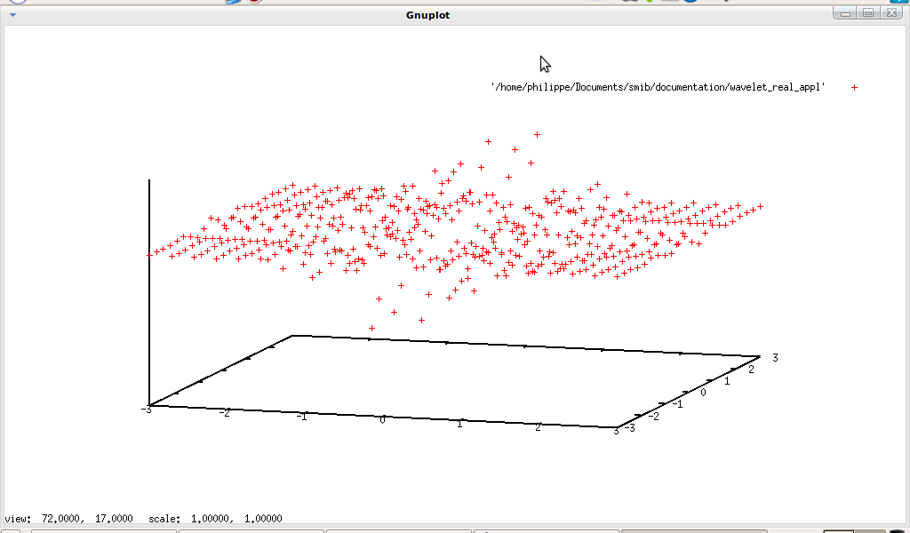
And for imaginary part:
5.5.6 Complex analysis↓
Now, we are going to see how to use Gauss scheme
↓↓ in the context of complex analysis.
First, how to draw a path in the complex plane
↓; the following program solves this problem:
gnuplotcomplexpath(P,N)=prog(C,t,a,b,temp1,temp2,temp3,temp4,do(
C=P[1],
t=P[2],
a=P[3],
b=P[4],
temp1=sample(C,t,a,b,N),
temp2=Sdecomp(Sreal(temp1),2),
temp3=Sdecomp(Simag(temp1),2),
temp4=Srecomp(temp2,temp3),
gnuplot2D(temp4)
))
Now we can test it on C = ((R − r)cos(t) + d.ccos((R − r)t⁄r)) + i((R − r)sin(t) − d.sin((R − r)t⁄r)), r = 3, R = 5, d = 5. So in smib:
a=0
b=6*pi
N=100
r=3
R=5
d=5
C=((R-r)cos(t)+d*cos((R-r)*t/r)+i*((R-r)sin(t)-d*sin((R-r)*t/r)),t,a,b)
Cur=gnuplotcomplexpath(C,N)
With qgfe:
 ↓↓↓
↓↓↓Complex path integral is defined by:
∫Cf(z).dz = ∫[a, b]f(C(t)).C’(t).dt,
C:[a, b] → ℂ; so in smib:
numcomplexpathint(f,z,P)=prog(C,t,a,b,temp1,do(
C=P[1],
t=P[2],
a=P[3],
b=P[4],
temp1=num(numint(subst(C,z,f)*d(C,t),t,a,b)),
return(temp1)
))
Let C = R.exp(it), R = 1, t ∈ [a, b], f(z) = 1⁄z, we want to check: ∫Cf(z).dz = 2iπ:
I=num(numcomplexpathint(f,z,C)-2*i*pi)
print("f =",f)
print("I =",I)
And smib gives:
f = 1/z
I = 0.00646429*i
If f(z) = log(z):
f = log(z)
I = -0.0203068 - 0.000138975 i
↓↓Index of a path is defined by: Ind(C, z0) = 1⁄2iπ∫C1⁄z − z0dz, so in smib:
numindex(P,z0)=prog(temp1,do(
temp1=num(numcomplexpathint(1/(z-z0),z,P)/(2*i*pi)),
return(temp1)
))
With this small script:
print("index")
z0=0
I=numindex(C,z0)
print("z0 =",z0," Index = ",I)
z0=2
I=numindex(C,z0)
print("z0 =",z0," Index = ",I)
z0=2*i
I=numindex(C,z0)
print("z0 =",z0," Index = ",I)
a=0
b=6*pi
r=3
R=5
d=5
C=((R-r)cos(t)+d*cos((R-r)*t/r)+i*((R-r)sin(t)-d*sin((R-r)*t/r)),t,a,b)
print("C =",C)
z0=0
I=numindex(C,z0)
print("z0 =",z0," Index = ",I)
z0=5
I=numindex(C,z0)
print("z0 =",z0," Index = ",I)
z0=-5
I=numindex(C,z0)
print("z0 =",z0," Index = ",I)
smib gives:
index
z0 = 0
Index = 1.00103
z0 = 2
Index = -0.00102839+5.37827e-17*i
z0 = 2*i
Index = 0.000213725+0.000456854*i
C = (2*cos(t)+5*cos(2/3*t)+2*i*sin(t)-5*i*sin(2/3*t),t,0,6*pi)
z0 = 0
Index = -2.00354-1.18686e-16*i
z0 = 5
Index = -1.13743-1.08772e-14*i
z0 = -5
Index = -0.500247-5.85538e-16*i
We can also compute number of singularities↓↓ NSing(f, C) = 1⁄2iπ∫Cf’⁄fdz, in smib:
numsing(f,z,P)=prog(temp1,do(
temp1=num(numcomplexpathint(simplify(d(f,z)/f),z,P)/(2*i*pi)),
return(temp1)
))
Using this test script:
print("number of singularities")
a=0
b=2*pi
R=2
C=(R*exp(i*t),t,a,b)
print("C =",C)
f=z^2+1
I=numsing(f,z,C)
print("f =",f," I =",I)
f=1/(1+z^2)
I=numsing(f,z,C)
print("f =",f," I =",I)
f=sin(z)
I=numsing(f,z,C)
print("f =",f," I =",I)
f=1/sin(z)
I=numsing(f,z,C)
print("f =",f," I =",I)
f=1/(1+z^3)
I=numsing(f,z,C)
print("f =",f," I =",I)
f=1+z^3
I=numsing(f,z,C)
print("f =",f," I =",I)
f=z-1
I=numsing(f,z,C)
print("f =",f," I =",I)
f=1/(z+1)
I=numsing(f,z,C)
print("f =",f," I =",I)
f=z-1+1/(z+1)
I=numsing(f,z,C)
print("f =",f," I =",I)
and smib gives:
number of singularities
C = (2*exp(i*t),t,0,2*pi)
f = 1+z^2
I = 2.00163+9.75002e-19*i
f = 1/(1+z^2)
I = -2.00163-9.75002e-19*i
f = sin(z)
I = 1.0023+2.13904e-16*i
f = 1/(sin(z))
I = -1.0023-2.13904e-16*i
f = 1/(1+z^3)
I = -3.00261-1.76267e-18*i
f = 1+z^3
I = 3.00261+1.76267e-18*i
f = -1+z
I = 1.00206+5.37827e-17*i
f = 1/(1+z)
I = -1.00053-3.39165e-17*i
f = -1+z+1/(1+z)
I = 1.00153-3.95706e-17*i
N.B.: the final result is not correct, another ↓weakness.
5.5.7 ↓Ordinary differential equation
With the operator
odesolve, smid can resolve symbolically ordinary differential equation↓ like: q(x)y’ + p(x)y = g(x) (smib simply applies: u(x) = e∫xp(t)⁄q(t)dt and y = (∫xu(t)g(t)⁄q(t)dt + c)⁄u(x)), or ay’’(x) + by’(x) + cy(x) = g(x) (smib computes solutions of homogeneous equation, then with some linear algebra (↓ wronskian) and two integrations it computes solutions. If a particular solution y0 is known, odesolve can also solve equation like a(x)y’’(x) + b(x)y’(x) + c(x)y(x) = g(x), the other solution of homogeneous equation is given by y1 = y0∫exp( − ∫b(x)⁄a(x)dx)⁄y20dx, the general solution is once again given using wronskian and some linear algebra. For examples :
f=quote(f)
C1=quote(C1)
C2=quote(C2)
Op(f,x)=d(f,x)-x*f-sin(x)
print("Op(f,x) = ",Op(f(x),x))
sol=odesolve(Op(f(x),x),f(x),x)
print("Sol = ",sol)
Op(sol,x)
f=quote(f)
C1=quote(C1)
C2=quote(C2)
print("Op(f,x) = ",Op(f(x),x))
Op(f,x)=d(f,x,2)+d(f,x)-2*f-sin(x)
sol=odesolve(Op(f(x),x),f(x),x)
print("Sol = ",sol)
simplify(factor(Op(sol,x)))
f=quote(f)
C1=quote(C1)
C2=quote(C2)
print("Op(f,x) = ",Op(f(x),x))
Op(f,x)=d(f,x,2)+2*d(f,x)+f+sin(x)
sol=odesolve(Op(f(x),x),f(x),x)
print("Sol = ",sol)
Op(sol,x)
f=quote(f)
C1=quote(C1)
C2=quote(C2)
print("Op(f,x) = ",Op(f(x),x))
Op(f,x)=d(f,x,2)-4*d(f,x)+5*f+sin(x)
sol=odesolve(Op(f(x),x),f(x),x)
print("Sol = ",sol)
simplify(factor(Op(sol,x)))
f=quote(f)
C1=quote(C1)
C2=quote(C2)
Op(f,x)=d(f,x)-x*f-h(x)
print("Op(f,x) = ",Op(f(x),x))
sol=odesolve(Op(f(x),x),f(x),x)
print("Sol = ",sol)
Op(sol,x)
f=quote(f)
C1=quote(C1)
C2=quote(C2)
Op(f,x)=d(f,x,2)+d(f,x)-2*f-h(x)
print("Op(f,x) = ",Op(f(x),x))
sol=odesolve(Op(f(x),x),f(x),x)
print("Sol = ",sol)
simplify(factor(Op(sol,x)))
f=quote(f)
C1=quote(C1)
C2=quote(C2)
Op(f,x)=d(f,x)-x*f-sgn(x)
print("Op(f,x) = ",Op(f(x),x))
sol=odesolve(Op(f(x),x),f(x),x)
print("Sol = ",sol)
Op(sol,x)
f=quote(f)
C1=quote(C1)
C2=quote(C2)
Op(f,x)=d(f,x,2)+d(f,x)-2*f-sgn(x)
print("Op(f,x) = ",Op(f(x),x))
sol=odesolve(Op(f(x),x),f(x),x)
print("Sol = ",sol)
simplify(factor(Op(sol,x)))
f=quote(f)
C1=quote(C1)
C2=quote(C2)
Op1(f,x)=d(f,x)-f
Op2(f,x)=d(f,x)+x*f
Op(f,x)=Op2(Op1(f,x),x)
f0=exp(x)
print("Op(f,x) = ",Op(f(x),x))
sol=odesolve(Op(f(x),x),f(x),x,f0)
print("Sol = ",sol)
simplify(factor(Op(sol,x)))
print(" ")
And smib gives :
Op(f,x) = d(f(x),x)-x*f(x)-sin(x)
1st order
Sol = C*exp(1/2*x^2)+exp(1/2*x^2)*integral(exp(-1/2*x^2)*sin(x),x)
0
Op(f,x) = d(f(x),x)-x*f(x)-sin(x)
2nd order : constant coefficient
Sol = -1/10*cos(x)+C1*exp(-2*x)+C2*exp(x)-3/10*sin(x)
0
Op(f,x) = d(d(f(x),x),x)+d(f(x),x)-2*f(x)-sin(x)
2nd order : constant coefficient
Sol = 1/2*cos(x)+C1*exp(-x)+C2*x*exp(-x)
0
Op(f,x) = d(d(f(x),x),x)+2*d(f(x),x)+f(x)+sin(x)
2nd order : constant coefficient
Sol=C1*exp(2*x-i*x)+C2*exp(2*x+i*x)
-1/2*i*exp(2*x-i*x)*integral(exp(-2*x)*sin(x)*sin(1/2*pi-x),x)
+1/2*i*exp(2*x+i*x)*integral(exp(-2*x)*sin(x)*sin(1/2*pi-x),x)
+1/2*exp(2*x-i*x)*integral(exp(-2*x)*cos(1/2*pi-x)*sin(x),x)
+1/2*exp(2*x+i*x)*integral(exp(-2*x)*cos(1/2*pi-x)*sin(x),x)
exp(-i*x)*(1/2*cos(x)*cos(1/2*pi-x)-cos(1/2*pi-x)*sin(x)-1/2*i*cos(x)*sin(1/2*pi-x)
-1/2*i*cos(1/2*pi-x)*sin(x)+1/2*i*exp(2*i*x)*cos(x)*sin(1/2*pi-x)
+1/2*i*exp(2*i*x)*cos(1/2*pi-x)*sin(x)-i*exp(2*i*x)*sin(x)*sin(1/2*pi-x)
+i*sin(x)*sin(1/2*pi-x)+1/2*exp(2*i*x)*cos(x)*cos(1/2*pi-x)
-exp(2*i*x)*cos(1/2*pi-x)*sin(x)
-1/2*exp(2*i*x)*sin(x)*sin(1/2*pi-x)+exp(i*x)*sin(x)-1/2*sin(x)*sin(1/2*pi-x))
Op(f,x) = d(f(x),x)-h(x)-x*f(x)
1st order
Sol = C*exp(1/2*x^2)+exp(1/2*x^2)*integral(exp(-1/2*x^2)*h(x),x)
0
Op(f,x) = d(d(f(x),x),x)+d(f(x),x)-2*f(x)-h(x)
2nd order : constant coefficient
Sol = C1*exp(-2*x)+C2*exp(x)
+1/3*exp(x)*integral(exp(-x)*h(x),x)-1/3*exp(-2*x)*integral(exp(2*x)*h(x),x)
0
Op(f,x) = d(f(x),x)-x*f(x)-sgn(x)
1st order
Sol = C*exp(1/2*x^2)+exp(1/2*x^2)*integral(exp(-1/2*x^2)*sgn(x),x)
0
Op(f,x) = d(d(f(x),x),x)+d(f(x),x)-2*f(x)-sgn(x)
2nd order : constant coefficient
Sol = C1*exp(-2*x)+C2*exp(x)+1/3*exp(x)*integral(exp(-x)*sgn(x),x)
-1/3*exp(-2*x)*integral(exp(2*x)*sgn(x),x)
0
Op(f,x) = d(d(f(x),x),x)-d(f(x),x)+x*d(f(x),x)-x*f(x)
2nd order : variable coefficient
Sol = C1*exp(x)+C2*pi^(1/2)*exp(1/2+x)*erf(x/(2^(1/2))+2^(-1/2))/(2^(1/2))
0
As the integrator is a little bit weak, ordinary differential equation can be also solved using numerical method, here we use Euler method↓↓ (Runge-Kutta method↓↓ is better... but harder to implement).
smib can solve the following global problem: dX(t)⁄dt = F(X(t)), X(a) = X0, t ∈ [a, b] where X is a scalar or a vector, Euler method can be implemanted as:
eulerode(F,X0,Var,Sample)=prog(a,b,n,dimpb,h,M,ind1,ind2,ind3,ind4,temp,do(
a=Sample[1],
b=Sample[2],
n=Sample[3],
dimpb=dim(Var),
h=(b-a)/n,
M=zero(n+1,dimpb),
for(ind1,1,n+1,M[ind1,1]=a+(ind1-1)*h),
for(ind1,1,n+1,
for(ind2,2,dimpb,
test(ind1==1,
test(dim(F)==0,M[ind1,ind2]=num(X0),
M[ind1,ind2]=num(X0[ind2-1])),
test(dim(F)==0,
do(temp=F,
for(ind3,1,dimpb,temp=subst(M[ind1-1,ind3],Var[ind3],temp)),
M[ind1,ind2]=num(M[ind1-1,ind2]+temp*h)),
do(temp=F,
for(ind3,1,dimpb,temp=subst(M[ind1-1,ind3],Var[ind3],temp)),
M[ind1,ind2]=num(M[ind1-1,ind2]+temp[ind2-1]*h)))))),
return(M)
))
For example, we want to solve the following differential equation:
df(x)⁄dx + 2f(x) = 2 − e − 4x, f(0) = 1
First symbolically:
odesolve(d(f(x),x)+2f(x)-2+exp(-4*x),f(x),x)
smib returns:
1+C*exp(-2*x)+1/2*exp(-4*x)
Now, we must compute C:
f=last
expand(subst(0,x,f)
smib gives:
3/2+C
Now we solve: 3⁄2 + C = 1:
roots(3/2+C=1,C)
smib answers:
-1/2
So the solution of df(x)⁄dx + 2f(x) = 2 − e − 4x, f(0) = 1 is f(x) = 1 − 1⁄2e − 2x + 1⁄2e − 4x.
Now numerically, with this script and qgfe:
f=2-exp(-4*x)-2*y
Var=(x,y)
Sample=(0,5,1000)
y0=1
gnuplot2D(eulerode(f,y0,Var,Sample))
quit()
We have:

Now we are going to study system of two differential equations
↓↓↓ like:
⎧⎨⎩
dtx(t) = F(x(t), y(t), t)
dty(t) = G(x(t), y(t), t)
x(0) = x0, y(0) = y0
A first classical example is the
↓↓Lotka-Volterra equation (predator-prey model
↓↓):
⎧⎨⎩
dtx(t) = x(t)(a − b.y(t))
dty(t) = y(t)( − c + d.x(t))
x(0) = x0, y(0) = y0
With the following script and qgfe:
a=3
b=1
c=2
d=1
LV=(x*(a-b*y),y*(-c+d*x))
X0=(8,4)
Var=(t,x,y)
Sp=(0,20,1000)
AS=eulerode(LV,X0,Var,Sp)
B=Sdecomp(AS,2)
C=Sdecomp(AS,3)
D=Srecomp(B,C)
gnuplot2D(D)
quit()
and we have:

We also can modify parameter, for example:
a=1
b=1
c=3
d=1
X0=(8,4)
then we have:

On the preceding examples, we only consider relation between
x and
y. But we can also use system of differential equation to solve higher order ordinary differential equation
↓↓↓, for example:
⎧⎨⎩
dtx(t) = y(t)
dty(t) = − x(t)
x(0) = 1, y(0) = 0
In fact this equation is equivalent to: d2tx(t) + x(t) = 0, x(0) = 0, x’(0) = 1,and analytical solution is x(t) = sin(t), so as usual:
A=(y,-x)
X0=(0,1)
Var=(t,x,y)
Sp=(0,10,1000)
AS=eulerode(A,X0,Var,Sp)
B=Sdecomp(AS,1)
C=Sdecomp(AS,2)
D=Srecomp(B,C)
gnuplot2D(D)
quit()
qgfe gives:

Once again, we must be suspicious, indeed, with this system:
⎧⎨⎩
dtx(t) = t.sin(x(t))
dty(t) = t.cos(y(t))
x(0) = 1, y(0) = 1
with the following script:
A=(sin(x)*t,cos(y)*t)
X0=(1,1)
Var=(t,x,y)
Sp=(0,100,1000)
AS=eulerode(A,X0,Var,Sp)
B=Sdecomp(AS,2)
C=Sdecomp(AS,3)
D=Srecomp(B,C)
gnuplot2D(D)
quit()
qgfe gives:
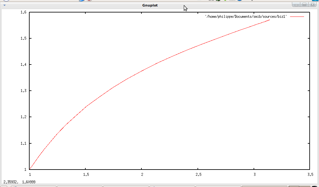
But if we enlarge time duration as in the following script:
A=(sin(x)*t,cos(y)*t)
X0=(1,1)
Var=(t,x,y)
Sp=(0,500,1000)
AS=eulerode(A,X0,Var,Sp)
B=Sdecomp(AS,2)
C=Sdecomp(AS,3)
D=Srecomp(B,C)
gnuplot2D(D)
quit()
We get the result below:

Astonishing, isn’t it!
We can also study
↓↓3D dynamic system.
First, Lorenz system
↓↓:
⎧⎪⎨⎪⎩
dx(t)⁄dt = σ.(y(t) − x(t))
dy(t)⁄dt = x(t).(ρ − z(t)) − y(t)
dz(t)⁄dt = x(t).y(t) − β.z(t)
x(0) = y(0) = z(0) = 1, β = 8⁄3, σ = 10, ρ = 28
So in smib:
beta=8/3
sigma=10
rho=28
f=(sigma*(y-x),x*(rho-z)-y,x*y-beta*z)
Var=(t,x,y,z)
Sample=(0,70,5000)
y0=(1,1,1)
A=eulerode(f,y0,Var,Sample)
gnuplot3D(Sdelete(A,1))
quit()
and qgfe gives:
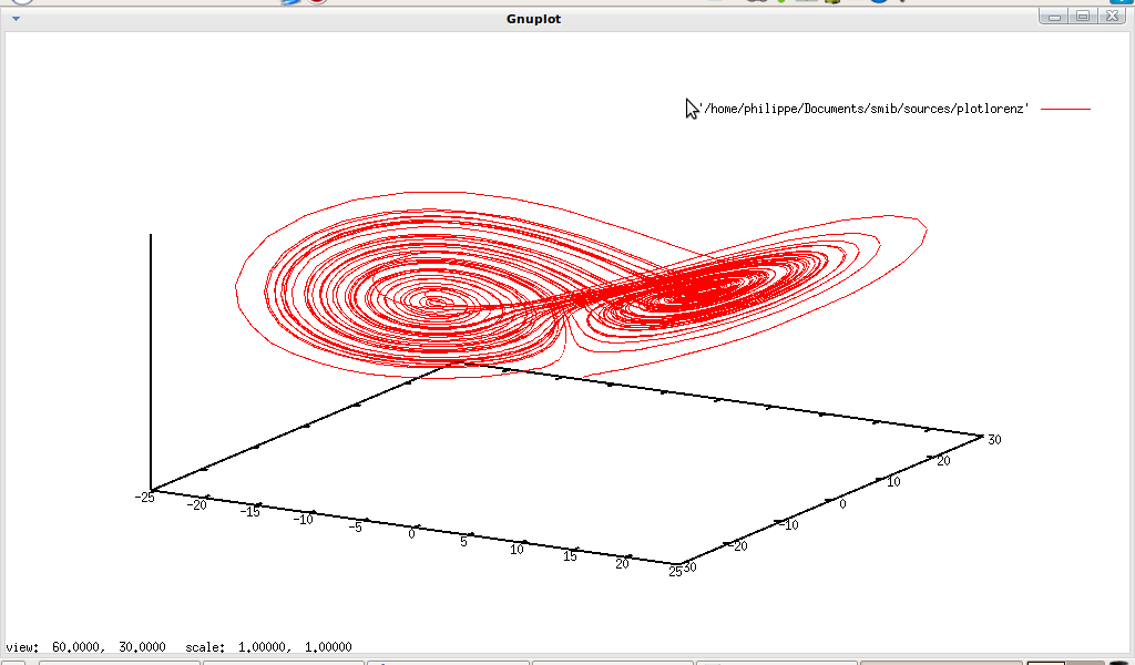
Or Rössler system
↓↓:
⎧⎪⎨⎪⎩
dx(t)⁄dt = − y(t) − z(t)
dy(t)⁄dt = x(t) + a.y(t)
dz(t)⁄dt = b + z(t).(x(t) − c)
x(0) = y(0) = z(0) = 1, a = b = 0.2, c = 5.7
So in smib:
a=0.2
b=0.2
c=5.7
f=(-y-z,x+a*y,b+z*(x-c))
Var=(t,x,y,z)
Sample=(0,200,5000)
y0=(1,1,1)
A=eulerode(f,y0,Var,Sample)
gnuplot3D(Sdelete(A,1))
quit()
and qgfe gives:
5.5.8 ↓Fractional calculus
Here, we want to compute
↓differintegration (
i.e. derivation of non-integer order
↓↓) of a function using Grünwald definition
↓:
dqf⁄d(x − x0)q = limN → ∞{[x − x0⁄N] − q⁄Γ( − q)∑j = N − 1j = 0Γ(j − q)⁄Γ(j + 1)f(x − j.[x − x0⁄N])}
So in smib:
numfracder1(f,x,q,x0,a,N)=((a-x0)/N)^(-q)/Gamma(-q)*
sum(ind,0,N-1,Gamma(ind-q)/Gamma(ind+1)*subst(a-ind*((a-x0)/N),x,f))
Some examples:
-
constant function f = 1, with q = 1⁄2:
symbolic solution is equal to 1⁄√(πx), using this script:
q=1/2
x0=0
N=20
f=1
gnuplot2D(sample(numfracder1(f,x,q,x0,a,N),a,1,10,50))
quit()
qgfe gives:

-
constant function f = 1, with q = − 1⁄2:
symbolic solution is equal to 2√(x⁄π), using this script:
q=-1/2
x0=0
N=20
f=1
gnuplot2D(sample(numfracder1(f,x,q,x0,a,N),a,1,10,50))
quit()
qgfe gives:
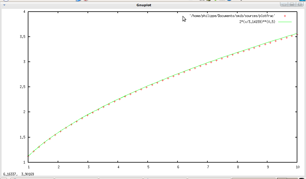
-
function f = arctan(√(x)), with q = 1⁄2:
symbolic solution is equal to √(π⁄1 + x)⁄2, using this script:
q=1/2
x0=0
N=20
f=arctan(sqrt(x))
gnuplot2D(sample(numfracder1(f,x,q,x0,a,N),a,1,10,50))
quit()
qgfe gives:
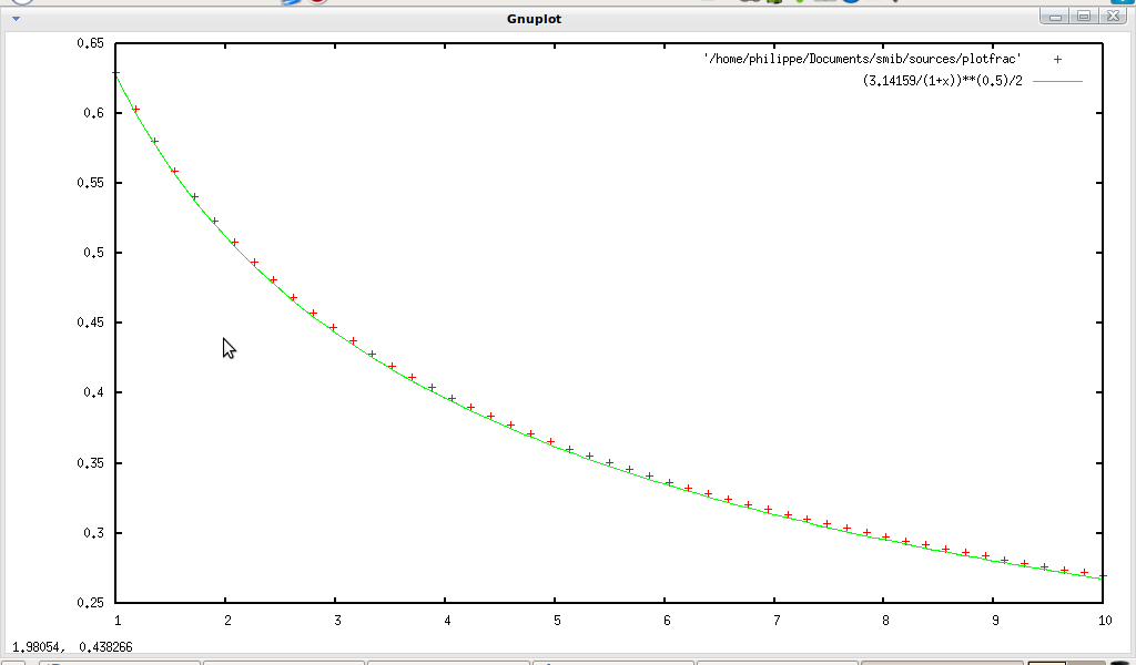
In fact, there exists a modified version of the Grünwald definition
↓↓:
dqf⁄d(x − x0)q = limN → ∞{[x − x0⁄N] − q⁄Γ( − q)∑j = N − 1j = 0Γ(j − q)⁄Γ(j + 1)f(x − (j − q⁄2).[x − x0⁄N])}
This definition is deemed to give an algorithm more efficient:
numfracder2(f,x,q,x0,a,N)=((a-x0)/N)^(-q)/Gamma(-q)*
sum(ind,0,N-1,Gamma(ind-q)/Gamma(ind+1)*subst(a-(ind-q/2)*((a-x0)/N),x,f))
We will study this.
-
On constant function:
f = 1, with q = 1⁄2: symbolic solution is equal to 1⁄√(πx), using this script:
f2=1
df12=1/sqrt(pi*x)
df22=2*sqrt(x/pi)
q=1/2
f=f2
df=df12
A=sample(numfracder1(f,x,q,x0,a,N),a,1,10,50)
B=sample(numfracder2(f,x,q,x0,a,N),a,1,10,50)
DF=sample(df,x,1,10,50)
print("Gap using 1st method: ",Snorm(Sdiff(A,DF)))
print("Gap using 2nd method: ",Snorm(Sdiff(B,DF)))
quit()
smib gives:
Gap using 1st method: (0.0396955,0.00525836,0.00180176)
Gap using 2nd method: (0.0396955,0.00525836,0.00180176)
constant function f = 1, with q = − 1⁄2: symbolic solution is equal to 2√(x⁄π), using this script:
f2=1
df12=1/sqrt(pi*x)
df22=2*sqrt(x/pi)
q=-1/2
f=f2
df=df22
A=sample(numfracder1(f,x,q,x0,a,N),a,1,10,50)
B=sample(numfracder2(f,x,q,x0,a,N),a,1,10,50)
DF=sample(df,x,1,10,50)
print("Gap using 1st method: ",Snorm(Sdiff(A,DF)))
print("Gap using 2nd method: ",Snorm(Sdiff(B,DF)))
quit()
And smib gives:
Gap using 1st method: (0.117733,0.0159192,0.00428559)
Gap using 2nd method: (0.117733,0.0159192,0.00428559)
For the constant function, there is no gain: it is not surprising because f is constant, and we only modify integration scheme.
-
On non constant function:
function f = arctan(√(x)), with q = 1⁄2: symbolic solution is equal to √(π⁄1 + x)⁄2, using this script:
q=1/2
x0=0
N=20
f1=arctan(sqrt(x))
df1=sqrt(pi/(1+x))/2
df2=sqrt(pi)*(sqrt(1+x)-1)
f=f1
df=df1
A=sample(numfracder1(f,x,q,x0,a,N),a,1,10,50)
B=sample(numfracder2(f,x,q,x0,a,N),a,1,10,50)
DF=sample(df,x,1,10,50)
print("Gap using 1st method: ",Snorm(Sdiff(A,DF)))
print("Gap using 2nd method: ",Snorm(Sdiff(B,DF)))
quit()
Then we have:
Gap using 1st method: (0.0181275,0.00253013,0.000204211)
Gap using 2nd method: (0.00925736,0.00129616,1.80853e-05)
function f = arctan(√(x)), with q = − 1⁄2: symbolic solution is equal to √(π)(√(1 + x) − 1), using this script:
q=-1/2
x0=0
N=20
f1=arctan(sqrt(x))
df1=sqrt(pi/(1+x))/2
df2=sqrt(pi)*(sqrt(1+x)-1)
f=f1
df=df2
A=sample(numfracder1(f,x,q,x0,a,N),a,1,10,50)
B=sample(numfracder2(f,x,q,x0,a,N),a,1,10,50)
DF=sample(df,x,1,10,50)
print("Gap using 1st method: ",Snorm(Sdiff(A,DF)))
print("Gap using 2nd method: ",Snorm(Sdiff(B,DF)))
quit()
Then we have:
Gap using 1st method: (0.116059,0.0157821,0.00387766)
Gap using 2nd method: (0.0132159,0.00165729,0.000823485)
function f = sin(√(x)), with q = 1⁄2: symbolic solution is equal to √(π)⁄2Jo(x), in a similar way:
Gap using 1st method: (7.20872,0.90126,0.454605)
Gap using 2nd method: (7.21362,0.901883,0.454891)
function f = sin(√(x)), with q = − 1⁄2: symbolic solution is equal to √(πx)J1(x):
Gap using 1st method: (14.0716,1.53183,1.23937)
Gap using 2nd method: (14.1149,1.54285,1.23535)
Here, we see that second method doesn’t always give better result, but when it works, it works fine, so in smib we use second definition.
We can also apply fractional calculus to samples.
Hereafter five examples:
-
f(x) = √(1 + x), q = 1⁄2, here derivative is: d1⁄2f(x) = 1⁄√(πx) + arctan(√(x))⁄√(π)
With the following script:
print("sqrt(1+x), q=1/2")
f=sample(sqrt(1+x),x,0,10,150)
q=1/2
qder(x)=num(Sfracd(f,q,x)-1/sqrt(pi*x)-arctan(sqrt(x))/sqrt(pi))
print("Gap:",Snorm(sample(qder,x,1,10,150)))
smib returns:
sqrt(1+x), q=1/2
Gap: (0.0612795,0.0034718,0.00357985)
-
f(x) = J0(√(x)), q = − 1⁄2, here derivative is: d − 1⁄2f(x) = 2sin(√(x))⁄√(π)
With the following script:
print("besselj(sqrt(x),0), q=-1/2")
f=sample(besselj(sqrt(x),0),x,0,10,150)
q=-1/2
qder(x)=num(Sfracd(f,q,x)-2*sin(sqrt(x))/sqrt(pi))
print("Gap:",Snorm(sample(qder,x,1,10,150)))
smib returns:
besselj(sqrt(x),0), q=-1/2
Gap: (0.0984872,0.00676304,0.00430091)
-
f(x) = J0(√(x)), q = 1⁄2, here derivative is: d1⁄2f(x) = cos(√(x))⁄√(πx)
With the following script:
print("besselj(sqrt(x),0), q=1/2")
f=sample(besselj(sqrt(x),0),x,0,10,150)
q=1/2
qder(x)=num(Sfracd(f,q,x)-cos(sqrt(x))/sqrt(pi*x))
print("Gap:",Snorm(sample(qder,x,1,10,150)))
smib returns:
besselj(sqrt(x),0), q=1/2
Gap: (0.0465338,0.00206661,0.00317324)
-
For f(x) = 1, we want to verify d1⁄2(d1⁄2)f = df = 0:
With the following script:
N=170
a=0
b=50
f1=1
q=1/2
print(" f=",f1,", q=",q,", a=",a,", b=",b,", N=",N)
f=sample(f1,x,a,b,N)
qder(x)=num(Sfracd(f,q,x))
S1=sample(qder,x,a+1,b,N)
print(" f=",f1,", q=1")
qder2(x)=num(Sfracd(S1,q,x))
S2=sample(qder2,x,a+2,b,N)
Sth=sample(d(f1,x),x,a+2,b,N)
print("Err=",Snorm(Sdiff(S2,Sth)))
gnuplot2D(Sdiff(S2,Sth))
smib gives:
f= 1 , q= 1/2 , a= 0 , b= 50 , N= 170
f= 1 , q=1
Err= (0.299963,0.00844421,0.021328)
Here we plot error:

-
For f(x) = 1, we want to verify d − 1⁄2(d1⁄2)f = f:
With the following script:
N=170
a=0
b=100
f1=1
q=1/2
f=sample(f1,x,a,b,N)
qder(x)=num(Sfracd(f,q,x))
S1=sample(qder,x,a+1,b,N)
qder2(x)=num(Sfracd(S1,-q,x))
S2=sample(qder2,x,a+2,b,N)
gnuplot2D(S2)
smib gives: (here result is not very good...)
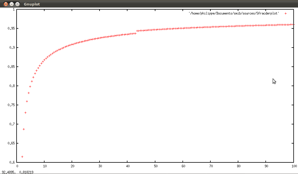
N.B.:
-
For a sample, fractional derivative computation could not start at beginning of sample, because there is not enough informations.
-
Number of sampling points could not exceed 170, because Γ function does not accept a greater argument (another ↓weakness).
5.6 Probalility↓ & statistic↓
5.6.1 ↓Distributions
5.6.2 ↓↓Distribution function
How to compute FP(x) = ∫[ − ∞, x]P(X)dX:
discretedistributionfunction(P,x,y)=num(sum(ind,0,ceiling(y),subst(ind,x,P)))
continousdistributionfunction(P,x,y)=numint(P,x,minfty,y)
5.6.3 ↓Moment, ↓variance
How to compute EP, X0, r = ∫ℝ(X − X0)rP(X)dX , EP, r = ∫ℝXrP(X)dX, EP, r, || = ∫ℝ|X|rP(X)dX:
discretecentermoment(P,x,y,r)=num(sum(ind,0,precdisc,subst(ind,x,(x-y)^r*P)))
discretemoment(P,x,r)=discretecentermoment(P,x,0,r)
discreteabsolutemoment(P,x,r)=num(sum(ind,0,precdisc,subst(ind,x,abs(x)^r*P)))
continouscentermoment(P,x,y,r)=numint((x-y)^r*P,x,minfty,infty)
continousmoment(P,x,r)=continouscentermoment(P,x,0,r)
continousabsolutemoment(P,x,r)=numint(abs(x)^r*P,x,minfty,infty)
statcentermoment(X,y,r)=num(sum(ind,1,dim(X),(X[ind]-y)^r)/dim(X))
statmoment(X,r)=statcentermoment(X,0,r)
statcovariance(X)=sum(ind,1,dim(X),(X[ind,1]-statmoment(Sdecomp(X,1),1))*
(X[ind,2]-statmoment(Sdecomp(X,2),1)))/dim(X)
5.6.4 Skewness↓, kurtosis↓
How to compute sk(P) = EP, EP, 0, 1, 3⁄E3⁄2P, EP, 0, 1, 2, ku(P) = EP, EP, 0, 1, 4⁄E2P, EP, 0, 1, 2 − 3
discreteskewness(P,x)=discretecentermoment(P,x,discretecentermoment(P,x,0,1),3)
/discretecentermoment(P,x,discretecentermoment(P,x,0,1),2)^(3/2)
discretekurtosis(P,x)=discretecentermoment(P,x,discretecentermoment(P,x,0,1),4)
/discretecentermoment(P,x,discretecentermoment(P,x,0,1),2)^2-3
continousskewness(P,x)=continouscentermoment(P,x,continouscentermoment(P,x,0,1),3)/
continouscentermoment(P,x,continouscentermoment(P,x,0,1),2)^(3/2)
continouskurtosis(P,x)=continouscentermoment(P,x,continouscentermoment(P,x,0,1),4)/
continouscentermoment(P,x,continouscentermoment(P,x,0,1),2)^2-3
5.6.5 ↓Linear least squares fitting
Here is a small program which computes least square line:
statleastsquare(X)=prog(temp1,temp2,temp3,temp4,temp5,temp6,do(
temp1=zero(3),
temp2=statcovariance(X),
temp3=statmoment(Sdecomp(X,1),1),
temp4=statmoment(Sdecomp(X,2),1),
temp5=statcentermoment(Sdecomp(X,1),temp3,2),
temp6=statcentermoment(Sdecomp(X,2),temp4,2),
temp1[1]=temp2/temp5,
temp1[2]=temp4-temp1[1]*temp3,
temp1[3]=temp2/sqrt(temp5*temp6),
return(temp1)
))
5.6.6 ↓Median & quantile↓
We compute quantile of continous distribution using dichotomic principle:
continousquantile(f,x,a,b,y)=
prog(temp0,temp1,temp2,temp3,temp4,temp5,temp6,do(
test(b==nil,temp0=-numinfty,temp0=b),
test(y==nil,temp6=numinfty,temp6=y),
temp1=numint(f,x,minfty,temp0)-a,
temp2=numint(f,x,minfty,(temp0+temp6)/2)-a,
temp3=numint(f,x,minfty,temp6)-a,
temp4=temp1*temp2,
temp5=temp2*temp3,
test(abs(temp2) < precision,(temp0+temp6)/2,
test(and(temp4 < 0,temp5 > 0),
quantile(f,x,a,(temp0+temp6)/2,temp0),
quantile(f,x,a,(temp0+temp6)/2,temp6)
))))
Median is computed as usual:
continousmedian(f,x)=quantile(f,x,1/2)
N.B.: continousquantile solves the following inversion problem↓: let F defined as F(x) = ∫xaf(x)dx, x ∈ [a, b], the problem is to find x such that F(x) = X.
5.6.7 Some examples
Some properties of distributions
Here we want to study expected value, variance, stantdard deviation, skewness, and kurtosis for some distribution:
n=quote(n)
x=quote(x)
print("bernoullidist: ",bernoullidist(n,1/3))
P=bernoullidist(n,1/3)
print("expected value: ",discretemoment(P,n,1))
print("variance: ",discretecentermoment(P,n,discretemoment(P,n,1),2))
print("standard deviation: ",
sqrt(discretecentermoment(P,n,discretemoment(P,n,1),2)))
print("skewness: ",discreteskewness(P,n))
print("kurtosis: ",discretekurtosis(P,n))
print(" ")
print("geometricdist: ",geometricdist(n,1/2))
P=geometricdist(n,1/2)
print("expected value: ",discretemoment(P,n,1))
print("variance: ",discretecentermoment(P,n,discretemoment(P,n,1),2))
print("standard deviation: ",
sqrt(discretecentermoment(P,n,discretemoment(P,n,1),2)))
print("skewness: ",discreteskewness(P,n))
print("kurtosis: ",discretekurtosis(P,n))
print(" ")
print("poissondist: ",poissondist(n,1/2))
P=poissondist(n,1/2)
print("expected value: ",discretemoment(P,n,1))
print("variance: ",discretecentermoment(P,n,discretemoment(P,n,1),2))
print("standard deviation: ",
sqrt(discretecentermoment(P,n,discretemoment(P,n,1),2)))
print("skewness: ",discreteskewness(P,n))
print("kurtosis: ",discretekurtosis(P,n))
print(" ")
print("uniformdist: ",uniformdist(x,0,1))
P=uniformdist(x,0,1)
print("expected value: ",continousmoment(P,x,1))
print("variance: ",continouscentermoment(P,x,continousmoment(P,x,1),2))
print("standard deviation: ",
sqrt(continouscentermoment(P,x,continousmoment(P,x,1),2)))
print("skewness: ",continousskewness(P,x))
print("kurtosis: ",continouskurtosis(P,x))
print(" ")
print("normaldist: ",normaldist(x,0,1))
P=normaldist(x,0,1)
print("expected value: ",continousmoment(P,x,1))
print("variance: ",continouscentermoment(P,x,continousmoment(P,x,1),2))
print("standard deviation: ",
sqrt(continouscentermoment(P,x,continousmoment(P,x,1),2)))
print("skewness: ",continousskewness(P,x))
print("kurtosis: ",continouskurtosis(P,x))
print(" ")
print("logisticdist: ",logisticdist(x,1,1))
P=logisticdist(x,1,1)
print("expected value: ",continousmoment(P,x,1))
print("variance: ",continouscentermoment(P,x,continousmoment(P,x,1),2))
print("standard deviation: ",
sqrt(continouscentermoment(P,x,continousmoment(P,x,1),2)))
print("skewness: ",continousskewness(P,x))
print("kurtosis: ",continouskurtosis(P,x))
print(" ")
print("laplacedist: ",laplacedist(x,1,1))
P=laplacedist(x,1,1)
print("expected value: ",continousmoment(P,x,1))
print("variance: ",continouscentermoment(P,x,continousmoment(P,x,1),2))
print("standard deviation: ",
sqrt(continouscentermoment(P,x,continousmoment(P,x,1),2)))
print("skewness: ",continousskewness(P,x))
print("kurtosis: ",continouskurtosis(P,x))
print(" ")
print("cauchydist: ",cauchydist(x,1,1))
P=cauchydist(x,1,1)
print("expected value: ",continousmoment(P,x,1))
print("variance: ",continouscentermoment(P,x,continousmoment(P,x,1),2))
print("standard deviation: ",
sqrt(continouscentermoment(P,x,continousmoment(P,x,1),2)))
print("skewness: ",continousskewness(P,x))
print("kurtosis: ",continouskurtosis(P,x))
print(" ")
X=(0,1,2,3,4,5)
print("X = ",X)
print("statmoment(X,1) = ",statmoment(X,1))
print("statcentermoment(X,statmoment(X,1),2) = ",
statcentermoment(X,statmoment(X,1),2))
print(" ")
Hereafter, we study least square fitting on sample with noise:
print("statleastsquare: ",4*x-33," with noise")
X=sample(4*x-33,x,-10,10,100)
Y=noisevector(dim(X))
Z=Sdecomp(X,1)
A=Sscalarproduct(1/10,Srecomp(Z,Y))
A=Ssum(X,A)
statleastsquare(A)
print(" ")
Last but not least, we test quantile and median:
f=normaldist(x,0,1)
A=1/5
print("quantile: f = ",f,", A = ",A)
B=continousquantile(f,x,A)
C=continousdistributionfunction(f,x,B)
print("quantile = ",B,", erreur = ",abs(C-A))
print(" ")
A=1/3
print("quantile: f = ",f,", A = ",A)
B=continousquantile(f,x,A)
C=continousdistributionfunction(f,x,B)
print("quantile = ",B,", erreur = ",abs(C-A))
print(" ")
print("median: f = ",f)
B=continousmedian(f,x)
C=continousdistributionfunction(f,x,B)
print("mediane = ",B,", erreur = ",abs(C-1/2))
print(" ")
f=studenttdist(x,1)
print("median: f = ",f)
B=continousmedian(f,x)
C=continousdistributionfunction(f,x,B)
print("median = ",B,", error = ",abs(C-1/2))
print(" ")
f=studenttdist(x,2)
print("median: f = ",f)
B=continousmedian(f,x)
C=continousdistributionfunction(f,x,B)
print("median = ",B,", error = ",abs(C-1/2))
print(" ")
f=studentzdist(x,1)
print("median: f = ",f)
B=continousmedian(f,x)
C=continousdistributionfunction(f,x,B)
print("median = ",B,", error = ",abs(C-1/2))
print(" ")
f=studentzdist(x,2)
print("median: f = ",f)
B=continousmedian(f,x)
C=continousdistributionfunction(f,x,B)
print("median = ",B,", error = ",abs(C-1/2))
print(" ")
And smib gives:
bernoullidist: 2/3*dirac(n)+1/3*dirac(1-n)
expected value: 0.333333
variance: 0.222222
standard deviation: 0.471405
skewness: 0.707107
kurtosis: -1.5
geometricdist: 1/2*(1/2)^n
expected value: 1
variance: 2
standard deviation: 1.41421
skewness: 2.12132
kurtosis: 6.5
poissondist: (1/2)^n*exp(-1/2)/n!
expected value: 0.5
variance: 0.5
standard deviation: 0.707107
skewness: 1.41421
kurtosis: 2
uniformdist: heaviside(x)-heaviside(-1+x)
expected value: 0.5
variance: 0.0833333
standard deviation: 0.288675
skewness: 1.99988e-15
kurtosis: -1.2
normaldist: exp(-1/2*x^2)/(2^(1/2)*pi^(1/2))
expected value: 8.49212e-18
variance: 1
standard deviation: 1
skewness: -3.19667e-17
kurtosis: 3.10862e-15
logisticdist: exp(1-x)/((1+exp(1-x))^2)
expected value: 1
variance: 3.28987
standard deviation: 1.8138
skewness: 2.24028e-15
kurtosis: 1.2
laplacedist: 1/2*exp(-abs(1-x))
expected value: 1
variance: 2
standard deviation: 1.41421
skewness: -1.17711e-06
kurtosis: 2.99998
cauchydist: 1/(pi*(2-2*x+x^2))
expected value: 0.987268
variance: 62.6683
standard deviation: 7.91633
skewness: -0.123486
kurtosis: 51.0329
X = (0,1,2,3,4,5)
statmoment(X,1) = 2.5
statcentermoment(X,statmoment(X,1),2) = 2.91667
statleastsquare: -33+4*x with noise
3.99894
-33.0014
0.999997
N.B.: Here the last component of the vector is the correlation coefficient↓↓.
quantile: f = exp(-1/2*x^2)/(2^(1/2)*pi^(1/2)) , A = 1/5
quantile = -0.842285 , error = 0.000185822
quantile: f = exp(-1/2*x^2)/(2^(1/2)*pi^(1/2)) , A = 1/3
quantile = -0.43335 , error = 0.000952933
median: f = exp(-1/2*x^2)/(2^(1/2)*pi^(1/2))
median = 0 , error = 1.22125e-15
median: f = x^2/pi+1/pi
median = -99.9998 , error = 0.000455474
median: f = (1+1/2*x^2)^(3/2)/(2*2^(1/2))
median = -100 , error = 0.000736037
median: f = (1+x^2)^(-1/2)
median = -60.6445 , error = 9.77535e-05
median: f = 2/(pi*(1+x^2))
median = -0.982666 , error = 0.000800322
Some applications of probability
Probalility and geometry
Let x and y two random numbers in [0, 1], what is the probalility of x2 + y2 ≤ 1 ?
Let X and Y random variables associated to x and y, so densities are: f1(x) = 1[0, 1](x) and f2(y) = 1[0, 1](y). As variables are independant, joint probability is f(x, y) = f1(x)f2(y). Hence probability is given by I = P(X2 + Y2 ≤ 1) = ∬Rdxdy = ∫[0, 1] × [0, π⁄2]rdrdθ.
We can use smib to compute I, and we have the following script:
I=defint(defint(r,theta,0,pi/2),r,0,1)
print("I=",I)
And the result is:
I= 1/4*pi
Probability and medicine
Let A a population of 2000 people, if the probability of an allergical reaction after an injection is 0,001.
-
What is the probability that 3 people will be ill ?
-
What is the probability that at least 2 people will be ill ?
Let
X the number of ill people,
X follows Poisson law
↓ i.e.:
P(X = x, λ) = λxe − λ⁄x!, λ = np = 2000*0, 001 = 2.
First question: A = P(X = 3, λ)
Second question: B = 1 − ∑a = 2a = 0P(X = a, λ)
So in smib:
lambda=2000*0.001
P(x,lambda)=lambda^x*exp(-lambda)/x!
A=P(3,lambda)
print("A=",A)
B=1-(sum(ind,0,2,P(ind,lambda)))
print("B=",B)
And smib gives:
A= 0.180447
B= 0.323324
Let
Yn = ∑i = ni = 1Xn, where
Xi is an infinite sequence of independent and identically distributed integrable random variables with expected value
E(X1) = μ, we want to verify that :
limn → ∞Yn⁄n = μ. We test it for coin-tossing
↓, exponential distribution with parameter equaling 1, and normal distribution with null mean and variance equaling 1; we test it for
n ∈ {1000, 10000, 30000}. For
n = 1000, the code is :
n=1000
s=1
SCT=Vcointoss(n)
MCT=num(sum(ind,1,dim(SCT),SCT[ind])/n)
SN=normnoisevector(n,s)
MN=sum(ind,1,dim(SN),SN[ind])/n
SE=exponentialnoisevector(n,1)
ME=sum(ind,1,dim(SE),SE[ind])/n
print("n = ",n)
print("MCT = ", MCT)
print("MN = ", MN)
print("ME = ", ME)
And smib gives :
n = 1000
MCT = 0.478
MN = 0.0148848
ME = 0.982549
n = 10000
MCT = 0.4985
MN = 0.00241706
ME = 0.996672
n = 30000
MCT = 0.4973
MN = 0.0113651
ME = 1.00112
real 1m7.549s
user 1m1.348s
sys 0m2.404s
Central limit theorem
↓↓: visual approach
Here we use the notion of
↓histogram to aggregate experimental data. Then we will use this aggregate to compare the theoretical result. We simply use coin-tossing (one of the simplest program
cointoss()=test(random()<1/2,0,1)), Xnis the corresponding random variable. Let Yn = ∑i = ni = 1Xn, we want to study the behaviour of the following sequence : (Yn − n⁄2)⁄√(n)⁄2. As infity is unreachable, we stop computation at n = 1000, and the experience is reapeted 5000 times. Then with the following programs :
CLT(n,m)=prog(ind1,ind2,Sn,temp,do(
temp=zero(m),
Sn=zero(n),
for(ind1,1,n,do(
temp=Vcointoss(m),
Sn[ind1]=num((sum(ind2,1,dim(temp),temp[ind2])-m/2)/(sqrt(m)/2))
)),
return(Sn)
))
and:
Vcointoss(n)=prog(temp,do(
temp=zero(n),
for(ind,1,n,temp[ind]=cointoss()),
return(temp)
))
So with the following script :
A=CLT(5000,1000)
I=(-5,5)
Sh=Shistogram(A,I)
gnuplot2D(Sh)
Using histogram an qgfe :
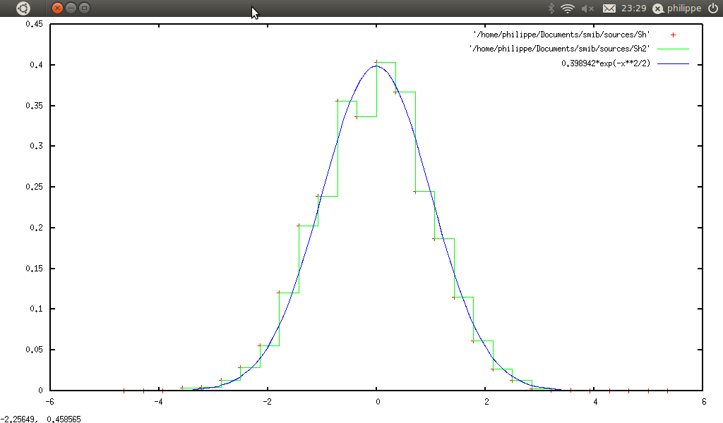
Computation is relatively long :
real 6m22.648s
user 6m20.876s
sys 0m0.272s
the coin is tossed 5000000 times.
We can do the same with ↓↓exponential distribution. We generate a vector of random numbers of this type using the following program :
exponentialnoisevector(n,sigma)=prog(temp0,temp1,do(
temp1=zero(n),
for(temp0,1,n,temp1[temp0]=num(-log(random())/sigma)),
return(temp1)
))
We choose σ = 1⁄2, theory gives :
-
mean = 1⁄σ
-
variance =1⁄σ2
and Xn is our vector, we want to test if ∑i = ni = 1Xi − m⁄s⁄√(m⁄s) looks like normal distribution. As preceding, we stop computation at n = 600, and the experience is reapeted 800 times. Then with the following programs :
CLT(n,m,s)=prog(ind1,ind2,Sn,temp,do(
temp=zero(m),
Sn=zero(n),
for(ind1,1,n,do(
temp=exponentialnoisevector(m,s),
Sn[ind1]=num((sum(ind2,1,dim(temp),temp[ind2])-m/s)/sqrt(m/s^2))
)),
return(Sn)
))
and the script :
print("CLT")
s=1/2
m=600
A=CLT(800,m,s)
I=(-5,5)
Sh2=Shistogram(A,I)
gnuplot2D(Sh2)
And qgfe gives :
5.6.8 Random number generation
smib provides two types of random number
↓s, the first following a uniform distribution
↓, the other a normal distribution
↓. For uniform distribution we choose
rand function provided by g++, for normal random number we choose Box-Muller method↓↓. We will test this. Let A be a vector of uniform type (between − 1 and 1), B type normal (mean is null, variance equal to two). We calculate the mean↓, variance↓, skewness↓, kurtosis↓.
n=5000
A=noisevector(n)
B=normnoisevector(n,2)
print("statmoment(A,1) = ", statmoment(A,1))
print("statcentermoment(A,statmoment(A,1),2) = ", statcentermoment(A,statmoment(A,1),2))
print("statskewness(A) = ", statskewness(A))
print("statkurtosis(A) = ", statkurtosis(A))
print("statmoment(B,1) = ", statmoment(B,1))
print("statcentermoment(B,statmoment(B,1),2) = ", statcentermoment(B,statmoment(B,1),2))
print("statskewness(B) = ", statskewness(B))
print("statkurtosis(B) = ", statkurtosis(B))
smib gives:
statmoment(A,1) = -0.00231545
statcentermoment(A,statmoment(A,1),2) = 0.337485
statskewness(A) = -0.0130419
statkurtosis(A) = -1.21037
statmoment(B,1) = -0.00709527
statcentermoment(B,statmoment(B,1),2) = 1.96465
statskewness(B) = 0.0055657
statkurtosis(B) = -0.0624164
We find some properties of the uniform law for A, and the normal law for B.
Another way is to use ↓inversion method for random number (let C be cumulative distribution function of the law γ (C(x) = ∫x − ∞γ(t)dt); as 0 ≤ C(x) ≤ 1 ∀x if we choose y in [0, 1], then g:y⟼C − 1(y) generates random number following law γ). In fact we use the function Squantile which is a discrete version of quantile, the function support gives an approximation of the support↓ of the distribution; those two functions are not described here: cf. init.cpp :
randomgenerator(dist,x,n)=prog(supp,a,b,n,m,S,X,Y,do(
supp=support(dist,x),
a=supp[1],b=supp[2],
m=ceiling(b-a)*randomprec,
test(m<100,m=2*m),
S=sample(dist,x,a,b,m),
X=zero(n+1),
for(ind,1,n+1,X[ind]=num(random())),
Y=zero(n+1), for(ind,1,n+1,Y[ind]=Squantile(S,X[ind])),
Y
))
We can test quality of this generator. First we compute cumulative distribution function of the law γ, we compute histogram of list of random number, then empirical distribution function. Finally we compare these two distribution function. So in smib :
testrandomgenerator(Sr,dist,x)=prog(I,Sh,S1,S2,S3,A,do(
I=support(dist,x),
Sh=Shistogram(Sr,I),
S1=Secd(Sh),
S2=Sdist(dist,x,S1),
S3=Sabs(Sdiff(S1,S2)),
print(\"Snorm = \",Snorm(S3)),
))
On this small script :
verbmode=0
print(" ")
s=1/2
m=0
n=50
dist=normaldist(x,m,s)
print("dist = ",dist)
Sr1=randomgenerator(dist,x,n)
testrandomgenerator(Sr1,dist,x)
print(" ")
s=2
m=0
n=50
dist=normaldist(x,m,s)
print("dist = ",dist)
Sr1=randomgenerator(dist,x,n)
testrandomgenerator(Sr1,dist,x)
print(" ")
a=1
n=50
dist=maxwelldist(x,a)
print("dist = ",dist)
Sr1=randomgenerator(dist,x,n)
testrandomgenerator(Sr1,dist,x)
print(" ")
s=1/2
m=0
n=50
dist=lognormaldist(x,m,s)
print("dist = ",dist)
Sr1=randomgenerator(dist,x,n)
testrandomgenerator(Sr1,dist,x)
quit()
and smib gives :
dist = 2^(1/2)*exp(-2*x^2)/(pi^(1/2))
support = (-3.06022,3.06022)
Snorm = (0.130924,0.0181257,0.0299305)
dist = exp(-1/8*x^2)/(2*2^(1/2)*pi^(1/2))
support = (-11.7473,11.7473)
Snorm = (0.131343,0.014202,0.0321015)
dist = 2^(1/2)*x^2*exp(-1/2*x^2)/(pi^(1/2))
support = (-6.81145,6.81145)
Snorm = (2.48313,0.479522,0.458782)
dist = 2^(1/2)*exp(-2*log(x)^2)*heaviside(x)/(pi^(1/2)*x)
support = (-0.0987167,16.0908)
Snorm = (2.20476,0.567725,0.157799)
real 2m0.437s
user 1m58.731s
sys 0m0.604s
5.6.9 Classical approach using brownian motion ↓
Let
[a, b] ⊂ ℝ, we want to construct a brownian motion
↓ Bt on it. This problem is solved with the following program:
brownianmotion(a,b,n)=prog(ind,B,h,do(
h=(b-a)/n,
B=zero(n+1,2),
for(ind,1,n+1,B[ind,1]=a+(ind-1)*h),
for(ind,1,n+1,test(ind==1,B[ind,2]=0,
B[ind,2]=B[ind-1,2]+num(normrand(h)))),
return(B)
))
So if we want to simulate brownian motion on [0, 1] with 1000 steps and draw it, with the following script:
gnuplot2D(brownianmotion(0,1,1000))
quit()
So using qgfe as usual, we have:
5.6.10 stochastic differential equation↓↓↓
Now we want to study stochastic differential equation:
dXt = f(t, Xt)dt + g(t, Xt)dBt, X0 = x0
we give two algorithms:
-
↓Euler-Maruyama method↓: Xt≃Xr + f(r, Xr)(t − r) + g(r, X)(Bt − Br)
So in smib:
eulersde(f,g,t,x,x0,B)=prog(M,n,ind,do(
n=dim(B),
M=zero(n,2),
for(ind,1,n,M[ind,1]=B[ind,1]),
for(ind,1,n,
test(ind==1,M[ind,2]=x0,
M[ind,2]=M[ind-1,2]+
subst(M[ind-1,2],x,subst(B[ind-1,1],t,f))*(M[ind,1]-M[ind-1,1])+
subst(M[ind-1,2],x,subst(B[ind-1,1],t,g))*(B[ind,2]-B[ind-1,2]))),
return(M)
))
-
Milstein method↓↓: Xt = Xr + f(r, Xr)(t − r) + g(r, Xr)(Bt − Br) + ∂xg(r, Xr)g(r, Xr)((Bt − Br)2 − (t − r))/(2)
So in smib:
milsteinsde(f,g,t,x,x0,B)=prog(M,n,ind,gp,do(
n=dim(B),
M=zero(n,2),
gp=d(g,x),
for(ind,1,n,M[ind,1]=B[ind,1]),
for(ind,1,n,test(ind==1,M[ind,2]=x0,
M[ind,2]=M[ind-1,2]+subst(M[ind-1,2],x,subst(B[ind-1,1],t,f))*
(M[ind,1]-M[ind-1,1])+
subst(M[ind-1,2],x,subst(B[ind-1,1],t,g))*(B[ind,2]-B[ind-1,2])+
subst(M[ind-1,2],x,subst(B[ind-1,1],t,gp))*
subst(M[ind-1,2],x,subst(B[ind-1,1],t,g))*
((B[ind,2]-B[ind-1,2])^2-(M[ind,1]-M[ind-1,1]))/2)),
return(M)
))
Here after two examples:
-
Ornstein-Uhlenbeck process↓↓: dXt = − aXtdt + σdBt, X0 = x0
Here we choose a = 1, σ = 1 ⁄ 2, x0 = 1, t ∈ [0, 1], with the following script:
B=brownianmotion(0,1,1000)
f=-x
g=1/2
x0=1
gnuplot2D(eulersde(f,g,t,x,x0,B))
quit()
and with qgfe as usual, we have:
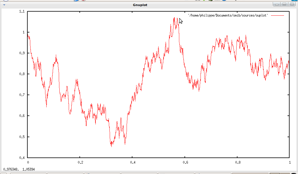
If we repeat the process tenfold, we get:
-
↓Black-Scholes-Merton process↓: dXt = μXtdt + σXtdBt, X0 = x0
Here we choose μ = 1 ⁄ 2, σ = 1 ⁄ 3, x0 = 1, t ∈ [0, 1], with the following script:
B=brownianmotion(0,1,1000)
f=x/2
g=x/3
x0=1
gnuplot2D(milsteinsde(f,g,t,x,x0,B))
quit()
and with qgfe, we have:
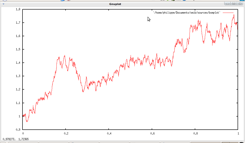
If we repeat the process tenfold, we get:
Now we can study average behavior of
Xt, we are going to see how to compute
E(Xt) and
Var(Xt) = E((Xt − E(Xt))2),
sk(Xt) (skewness
↓), and
ku(Xt) (kurtosis
↓).
First, we compute
n simulations of the equation on
m points; for this, we use the function multisde:
multisde(f,g,x0,x,I,M)=prog(B,X,a,b,m,n,ind,stoc,do(
a=I[1],b=I[2],m=M[1],n=M[2],stoc=M[4],
X=zero(n,m+1,2),
B=zero(m+1,2),
for(ind,1,n,do(
B=brownianmotion(a,b,m),
test(stoc==0,
X[ind]=eulersde(f,g,t,x,x0,B),
X[ind]=milsteinsde(f,g,t,x,x0,B))
)),
return(X)
))
Then we calculate the mean and variance with the function sdeanalysis:
sdeanalysis(f,g,x0,x,I,M)=prog(m,n,A,F,X,ind4,ind2,ind3,do(
m=M[1],n=M[2],nb=M[3],
A=zero(nb,4),
F=zero(m+1,5),
for(ind4,2,m+1,do(
for(ind2,1,nb,do(
X=multisde(f,g,x0,x,I,M),
Z=zero(n),
for(ind3,1,n,Z[ind3]=X[ind3,ind4,2]),
A[ind2,1]=statmoment(Z,1),
A[ind2,2]=statcentermoment(Z,A[ind2,1],2)
A[ind2,3]=statskewness(Z),
A[ind2,4]=statkurtosis(Z)
)),
F[ind4,1]=X[1,ind4,1],
F[ind4,2]=statmoment(transpose(A)[1],1),
F[ind4,3]=statmoment(transpose(A)[2],1),
F[ind4,4]=statmoment(transpose(A)[3],1),
F[ind4,5]=statmoment(transpose(A)[4],1)
)),
F[1,1]=X[1,1,1],
F[1,2]=x0,
F[1,3]=0,
F[1,4]=0,
F[1,5]=0,
return(F)
))
We can now apply this to brownian motion, sde is Xt = dBt, X0 = 0, t ∈ [0, 1], using Euler-Maruyama method script, can be:
a=0
b=1
f=a
g=b
x0=0
aI=0
bI=1
I=(aI,bI)
m=40
n=20
nb=20
stoc=0
M=(m,n,nb,stoc)
AN=num(sdeanalysis(f,g,x0,x,I,M,nb))
E=Sdelete(Sdelete(Sdelete(AN,5),4),3)
Var=Sdelete(Sdelete(Sdelete(AN,5),4),2)
sk=Sdelete(Sdelete(Sdelete(AN,5),3),2)
ku=Sdelete(Sdelete(Sdelete(AN,4),3),2)
print("E=",E)
print("Var=",Var)
print("sk=",sk)
print("ku=",ku)
Here theory gives E(Xt) = 0 and Var(Xt) = t, so with qgfe and gnuplot2D, we have:

For Ornstein-Uhlenbeck process
↓↓ dXt = − aXtdt + σdBt, X0 = x0 , with
a = 1, σ = 1 ⁄ 2, x0 = 1, t ∈ [0, 1] using Milstein method, we can use:
a=1
b=1/2
f=-a*x
g=b
x0=1
aI=0
bI=1
I=(aI,bI)
m=40
n=20
nb=20
stoc=1
M=(m,n,nb,stoc)
AN=num(sdeanalysis(f,g,x0,x,I,M,nb))
E=Sdelete(Sdelete(Sdelete(AN,5),4),3)
Var=Sdelete(Sdelete(Sdelete(AN,5),4),2)
sk=Sdelete(Sdelete(Sdelete(AN,5),3),2)
ku=Sdelete(Sdelete(Sdelete(AN,4),3),2)
Eth=exp(-a*x)
Varth=b^2/(2*a)*(1-exp(-2*a*x))
SEth=sample(Eth,x,aI,bI,m)
SVarth=sample(Varth,x,aI,bI,m)
print("ErrE=",Snorm(Sdiff(SEth,E)))
print("ErrVar=",Snorm(Sdiff(SVarth,Var)))
smib gives:
ErrE= (0.0988045,0.0107159,0.0111029)
ErrVar= (0.0336415,0.00398533,0.00342356)
With qgfe:
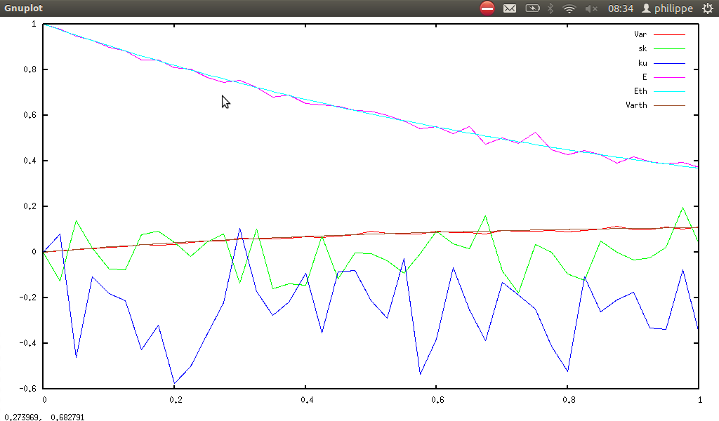
For
↓↓Vasicek process :
dXt = a.(b − Xt)dt + cXtdBt, X0 = x0, with
a = 3, b = 1⁄2, c = 1⁄3, t ∈ [0, 5], X0 = 3 using the following script :
a=3
b=1/2
c=1/3
f=a*(b-x)
g=c
x0=3
aI=0
bI=5
I=(aI,bI)
m=50
n=20
nb=20
stoc=1
M=(m,n,nb,stoc)
AN=num(sdeanalysis(f,g,x0,x,I,M,nb))
E=Sdelete(Sdelete(Sdelete(AN,5),4),3)
Var=Sdelete(Sdelete(Sdelete(AN,5),4),2)
sk=Sdelete(Sdelete(Sdelete(AN,5),3),2)
ku=Sdelete(Sdelete(Sdelete(AN,4),3),2)
Eth=x0*exp(-a*x)+b*(1-exp(-a*x))
Varth=c^2/(2*a)*(1-exp(-2*a*x))
SEth=sample(Eth,x,aI,bI,m)
SVarth=sample(Varth,x,aI,bI,m)
print("ErrE=",Snorm(Sdiff(SEth,E)))
print("ErrVar=",Snorm(Sdiff(SVarth,Var)))
smib gives:
ErrE= (0.380147,0.0277354,0.0454347)
ErrVar= (0.0170399,0.00206237,0.00119998)
With qgfe :
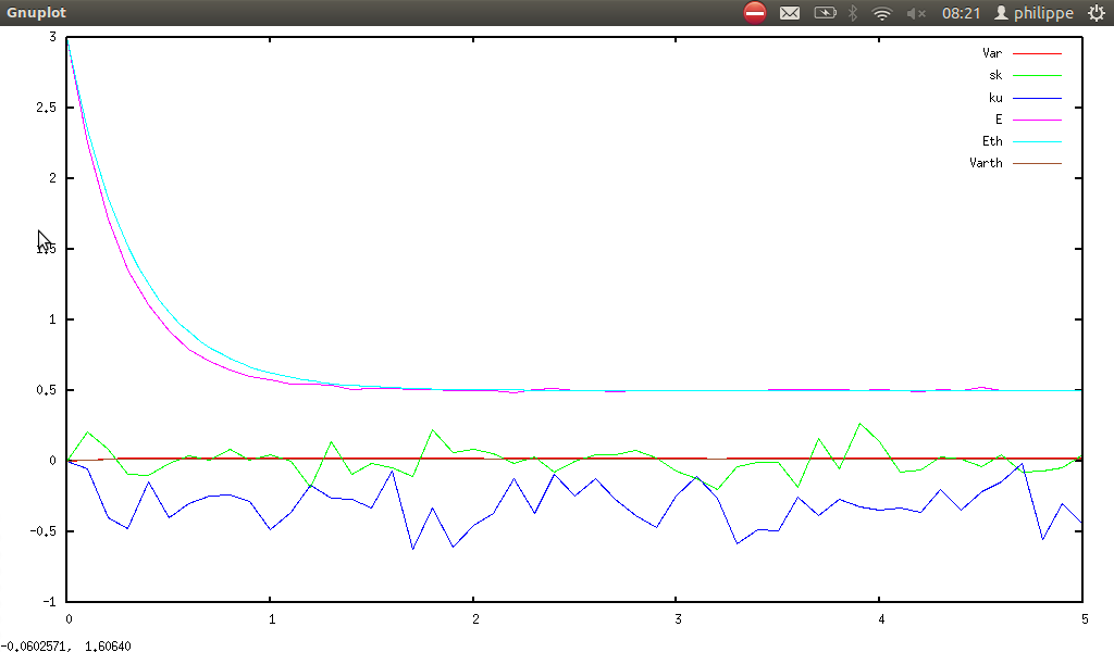
For Black-Scholes-Merton process
↓↓:
dXt = μXtdt + σXtdBt, X0 = 1, with
μ = 1 ⁄ 2, σ = 1 ⁄ 3, t ∈ [0, 1], using Euler-Maruyama method, script can be:
a=1/2
b=1/3
f=-a*x
g=b*x
x0=1
aI=0
bI=1
I=(aI,bI)
m=40
n=20
nb=20
stoc=0
M=(m,n,nb,stoc)
AN=num(sdeanalysis(f,g,x0,x,I,M,nb))
E=Sdelete(Sdelete(Sdelete(AN,5),4),3)
Var=Sdelete(Sdelete(Sdelete(AN,5),4),2)
sk=Sdelete(Sdelete(Sdelete(AN,5),3),2)
ku=Sdelete(Sdelete(Sdelete(AN,4),3),2)
Using smib and qgfe:
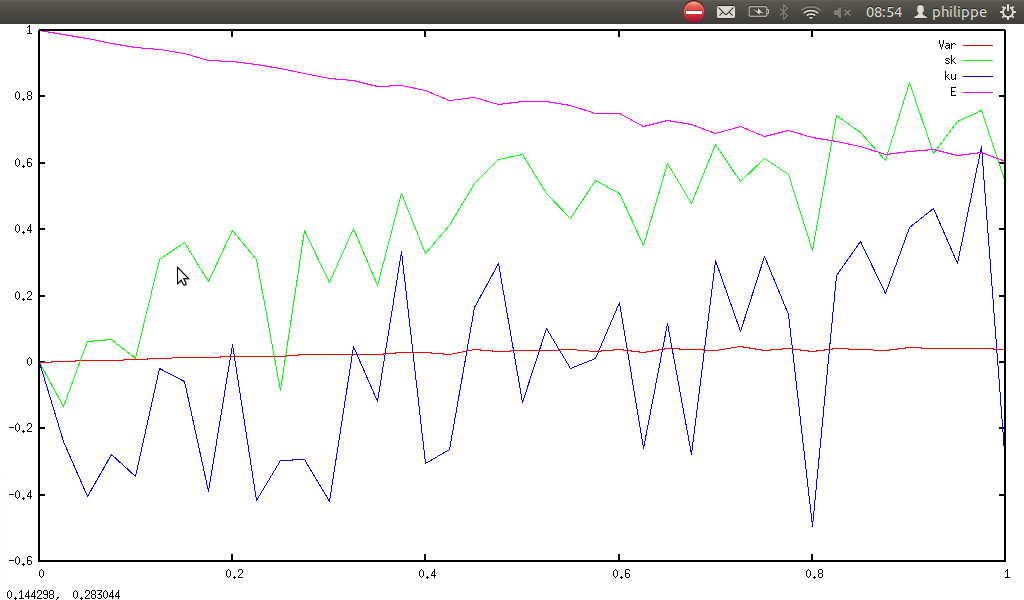
If we choose
m=80 (be patient) :
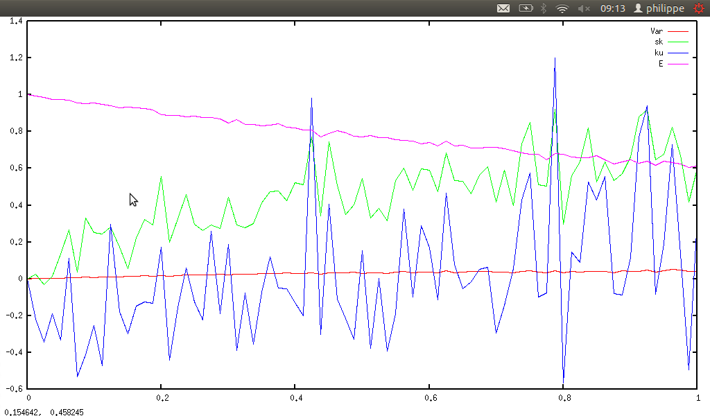
For
↓↓Cox-Ingersoll-Ross process :
dXt = a.(b − Xt)dt + c√(Xt)dBt, X0 = x0, with
a = 3, b = 1⁄2, c = 1⁄3, t ∈ [0, 5], X0 = 3 using the following script :
a=3
b=1/2
c=1/3
f=a*(b-x)
g=c*sqrt(x)
x0=3
aI=0
bI=5
I=(aI,bI)
m=50
n=20
nb=20
stoc=1
M=(m,n,nb,stoc)
AN=num(sdeanalysis(f,g,x0,x,I,M,nb))
E=Sdelete(Sdelete(Sdelete(AN,5),4),3)
Var=Sdelete(Sdelete(Sdelete(AN,5),4),2)
sk=Sdelete(Sdelete(Sdelete(AN,5),3),2)
ku=Sdelete(Sdelete(Sdelete(AN,4),3),2)
Eth=b+(x0-b)*exp(-a*x)
Varth=c^2/a*(1-exp(-a*x))*(x0*exp(-a*x)+b*(1-exp(-a*x))/2)
SEth=sample(Eth,x,aI,bI,m)
SVarth=sample(Varth,x,aI,bI,m)
print("ErrE=",Snorm(Sdiff(SEth,E)))
print("ErrVar=",Snorm(Sdiff(SVarth,Var)))
So smib gives :
ErrE= (0.369397,0.0269644,0.0441417)
ErrVar= (0.0204173,0.00175534,0.00225669)
Using qgfe :
5.6.11 Stratonovich calculus & Ito calculus
As Ito and Stratonovich calculi
↓ are equivalent, if we want to study:
dSt = f(St, t)dt + g(St, t)○dBt, we have the following equivalent formulation :
dSt = [f(St, t) + 1⁄2g(St, t)∂xg(St, t)]dt + g(St, t)dBt.
And thus
dSt = f(St, t)dt + g(St, t)dBt + h(St, t)○dBt is then equivalent to :
dSt = [f(St, t) + 1⁄2h(St, t)∂xh(St, t)]dt + [g(St, t) + h(St, t)]dBt.
The following script permits the convertion :
stratonovich2ito(F,X)=prog(G,f,g,h,x,t,do(
f=F[1],g=F[2],h=F[3],
x=X[1],t=X[2],
G=zero(2),
G[1]=f+1/2*h*d(h,x),
G[2]=g+h,
return(G)
))
Hereafter a first experience :
a=1/2
b=1/3
f=-a*x
g=0
h=b*x
F=(f,g,h)
X=(x,t)
G=stratonovich2ito(F,X)
f=G[1]
g=G[2]
x0=3
aI=0
bI=5
I=(aI,bI)
m=50
n=20
nb=20
stoc=1
M=(m,n,nb,stoc)
AN=num(sdeanalysis(f,g,x0,x,I,M,nb))
E=Sdelete(Sdelete(Sdelete(AN,5),4),3)
Var=Sdelete(Sdelete(Sdelete(AN,5),4),2)
print("E=",gnuplot2D(E))
print("Var=",gnuplot2D(Var))
With qgfe :
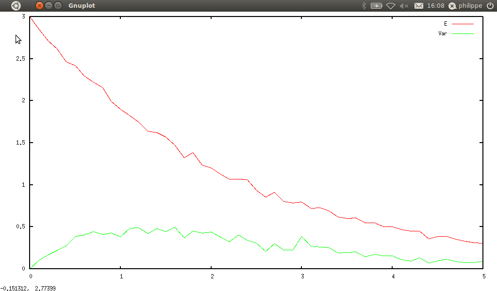
And a second with :
f=x
g=exp(-x^2)
h=sin(x)
gives:
5.6.12 Stochastic differential equation : generalized approach using inversion method
Here we want to study stochastic process defined by :
dXt = f(Xt, t)dt + g(Xt, t).dΓ, X0 = x0
where Γ is a stochastic process which is linked to law γ as brownian motion is linked to normal law.
Generation of random numbers using inversion formula is expensive so, as we assume that the numbers are generated independently, we can choose them uniformly from a list to generate random process :
Srandomprocess(S,a,b,n,m)=prog(ind1,ind2,ind3,B,h,do(
h=(b-a)/n,B=zero(m,n+1,2),
for(ind1,1,m,do(
for(ind2,1,n+1,B[ind1,ind2,1]=num(a+(ind2-1)*h)),
for(ind2,1,n+1,test(ind2==1,B[ind1,ind2,2]=0,
B[ind1,ind2,2]=B[ind1,ind2-1,2]+S[ceiling(num(random()*(dim(S))))]))
)),
B
))
We use ↓↓Euler-Maruyama method (this time, we do not use the Milstein method↓↓, because it directly uses the ↓Ito’s lemma, and we do not know how to compute explicitly the quadratic variation↓) :
eulergsde(F,X,x0,B)=prog(f,g,h,M,n,ind,do(
f=F[1],g=F[2],x=X[1],t=X[2],
n=dim(B),M=zero(n,2),
for(ind,1,n,M[ind,1]=B[ind,1]),
for(ind,1,n,test(ind==1,
M[ind,2]=x0,
M[ind,2]=num(M[ind-1,2]+
subst(M[ind-1,2],x,subst(B[ind-1,1],t,f))*(M[ind,1]-M[ind-1,1])+
(subst(M[ind-1,2],x,subst(B[ind-1,1],t,g)))*(B[ind,2]-B[ind-1,2])))),
return(M)
))
We generate multiple experiences:
Smultigsde(F,S,x0,X,I)=prog(B,SDE,Y,RD,a,b,m,n,f,g,dist,ind,do(
f=F[1],g=F[2],dist=F[3],a=I[1],b=I[2],n=I[3],m=I[4],
RD=zero(m,n+1,2),
SDE=zero(m,n+1,2),
B=zero(n+1,2),
RD=Srandomprocess(S,a,b,n,m),
for(ind,1,m,do(
B=RD[ind],
SDE[ind]=eulergsde(F,X,x0,B)
)),
SDE
))
Now we analyze the results:
Sgsdeanalysis(F,x0,X,I)=prog(f,g,h,dist,a,b,m,n,x,A,G,temp,S,ind4,ind2,ind3,do(
f=F[1],g=F[2],dist=F[3],x=X[1],a=I[1],b=I[2],n=I[3],m=I[4],nb=I[5],
print("X = ",X),
print("f = ",f),
print("g = ",g),
print("dist = ",dist),
print("a = ",a),
print("b = ",b),
print("number of points = ",n),
print("number of experiences = ",m),
print("number of groups = ",nb),
A=zero(nb,4),
G=zero(n+1,5),
S=randomgenerator(dist,x,n),
for(ind4,2,n+1,do(
print("Step = ",ind4),
for(ind2,1,nb,do(
temp=zero(m,n+1,2),
temp=Smultigsde(F,S,x0,X,I),
Z=zero(m),
for(ind3,1,m,Z[ind3]=temp[ind3,ind4,2]),
A[ind2,1]=statmoment(Z,1),
A[ind2,2]=statcentermoment(Z,A[ind2,1],2),
A[ind2,3]=statskewness(Z),
A[ind2,4]=statkurtosis(Z)
)),
G[ind4,1]=temp[1,ind4,1],
G[ind4,2]=statmoment(transpose(A)[1],1),
G[ind4,3]=statmoment(transpose(A)[2],1),
G[ind4,4]=statmoment(transpose(A)[3],1),
G[ind4,5]=statmoment(transpose(A)[4],1)
)),
G[1,1]=temp[1,1,1],
G[1,2]=x0,
G[1,3]=0,
G[1,4]=0,
G[1,5]=0,
G
))
We can try it on the simplest SDE in the world :Xt = dBt, X0 = 0, t ∈ [0, 1]. So in smib :
verbmode=0
N=30
aI=0
bI=1
X=(x,t)
a=3
b=1/2
c=1/3
f=0
g=1
x0=0
m=0
#number of points
n=N*(bI-aI)
s=sqrt((bI-aI)/n)
dist=normaldist(x,m,s)
#number of experiences
l=10
#number of groups
k=20
I=(aI,bI,n,l,k)
F=(f,g,dist)
AN=Sgsdeanalysis(F,x0,X,I)
E=Sdelete(Sdelete(Sdelete(AN,5),4),3)
Var=Sdelete(Sdelete(Sdelete(AN,5),4),2)
print("E=",E)
print("Var=",Var)
Eth=0
Varth=x
print("Eth = ",Eth)
print("Varth = ",Varth)
SEth=sample(Eth,x,aI,bI,n)
SVarth=sample(Varth,x,aI,bI,n)
print("ErrE=",Snorm(Sdiff(SEth,E)))
print("ErrVar=",Snorm(Sdiff(SVarth,Var)))
quit()
and smib gives :
X = (x,t)
f = 0
g = 1
dist = 3^(1/2)*5^(1/2)*exp(-15*x^2)/(pi^(1/2))
a = 0
b = 1
number of points = 30
number of experiences = 10
number of groups of experiences= 20
ErrE= (0.305133,0.0428106,0.034215)
ErrVar= (1.1961,0.183873,0.111089)
real 1m10.350s
user 1m8.900s
sys 0m0.320s
Using qgfe for plotting :
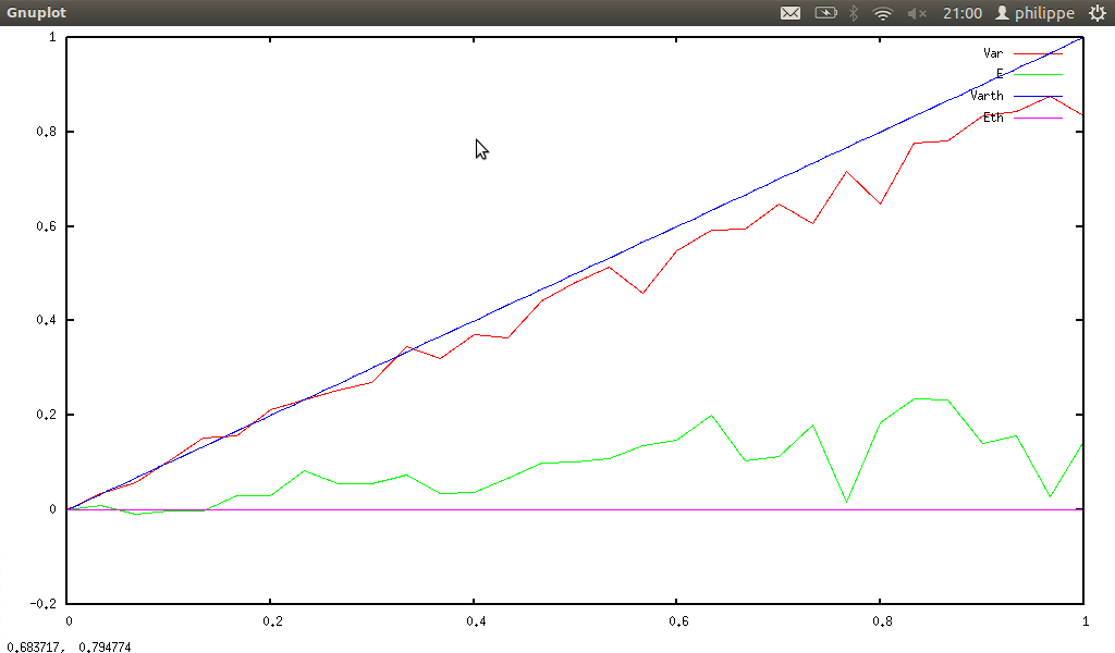
Another example :
verbmode=0
N=30
aI=0
bI=1
X=(x,t)
a=3
b=1/2
c=1/3
f=a*(b-x)
g=c*sqrt(x)
x0=0
m=0
#number of points
n=N*(bI-aI)
s=sqrt((bI-aI)/n)
dist=normaldist(x,m,s)
#number of experiences
l=10
#number of groups
k=20
I=(aI,bI,n,l,k)
F=(f,g,dist)
AN=Sgsdeanalysis(F,x0,X,I)
E=Sdelete(Sdelete(Sdelete(AN,5),4),3)
Var=Sdelete(Sdelete(Sdelete(AN,5),4),2)
print("E=",E)
print("Var=",Var)
Eth=b+(x0-b)*exp(-a*x)
Varth=c^2/a*(1-exp(-a*x))*(x0*exp(-a*x)+b*(1-exp(-a*x))/2)
print("Eth = ",Eth)
print("Varth = ",Varth)
SEth=sample(Eth,x,aI,bI,n)
SVarth=sample(Varth,x,aI,bI,n)
print("ErrE=",Snorm(Sdiff(SEth,E)))
print("ErrVar=",Snorm(Sdiff(SVarth,Var)))
quit()
smib gives :
X = (x,t)
f = 3/2-3*x
g = 1/3*x^(1/2)
dist = 3^(1/2)*5^(1/2)*exp(-15*x^2)/(pi^(1/2))
a = 0
b = 1
number of points = 30
number of experiences = 10
number of groups of experiences= 20
ErrE= (0.0358148,0.00519484,0.00379356)
ErrVar= (0.00679116,0.00102452,0.000661888)
real 1m8.220s
user 1m7.868s
sys 0m0.128s
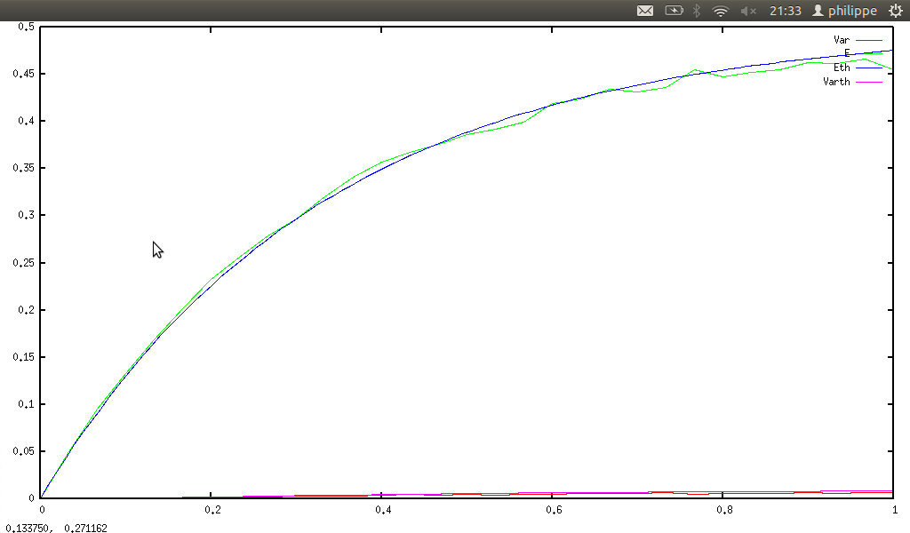
The generalized method offers mainly the possibility to choose a law other than the normal. For example we can choose the law of Fermi-Dirac↓↓ Γ, and we consider the following equation dXt = − aXtdt + σdΓt, X0 = x0 , with a = 1, σ = 1 ⁄ 2, x0 = 1, t ∈ [0, 2], so script is :
N=10,aI=0,bI=2
X=(x,t)
#number of points
n=N*(bI-aI)
#number of experiencess
l=10
#number of groups
k=10
a=-1,b=1/2,f=a*x,g=b
x0=1
m=0
s=sqrt((bI-aI)/n)
dist=fermidiracdist(x,m,s)
I=(aI,bI,n,l,k)
F=(f,g,dist)
AN=Sgsdeanalysis(F,x0,X,I)
E=Sdelete(Sdelete(Sdelete(AN,5),4),3)
Var=Sdelete(Sdelete(Sdelete(AN,5),4),2)
sk=Sdelete(Sdelete(Sdelete(AN,5),3),2)
ku=Sdelete(Sdelete(Sdelete(AN,4),3),2)
print("E=",E)
print("Var=",Var)
quit()
We only plot E and Var :
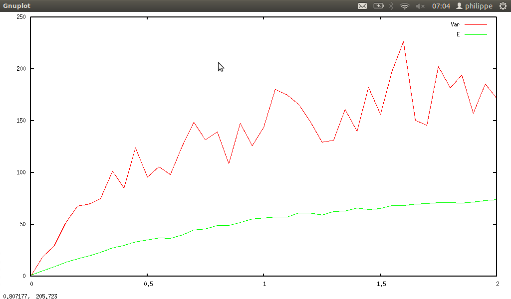
Same equation, but with lognormal distribution :
5.6.13 In higher dimension
Using odesolve we can solve symbolically an ordinary differential equation, with eulerode we treat them numerically; we can add some brownian motion... In fact we want to study \strikeout off\uuline off\uwave offdX(t) = F(X(t))dt + G(X(t))dBt, X(a) = X0, t ∈ [a, b], X is a scalar or a vector depending on t, F and G are functions depending on X. To do this, we just have to modify eulerode, adding random part, this gives the function eulerde (the code is in init.cpp).
-
\strikeout off\uuline off\uwave off↓↓Duffing-Van der Pool oscillator
⎧⎨⎩
dtx1(t) = x2(t)dt
dtx2(t) = (x1(t)(a − x1(t)2) − x2(t))dt + σx1(t)dBt
a = 1, σ = 0.5, x1(0) = 1, x2(0) = 1.
So in smib:
a=1
F=(x2,x1*(a-x1^2)-x2)
G=(0,0.5*x1)
X0=(1,1)
Var=(t,x1,x2)
Sp=(0,50,1000)
AS=eulerde(F,G,X0,Var,Sp)
B=Sdecomp(AS,2)
C=Sdecomp(AS,3)
D=Srecomp(B,C)
gnuplot2D(D)
Using qgfe :
If noise is reduced (\strikeout off\uuline off\uwave offσ = 0.01), we have :
-
↓↓Bonhoeffer Van der Pool oscillator
⎧⎨⎩
dtx1(t) = c(x1(t) + x2(t) − x31(t)⁄3 + z)dt + σdBt
dtx2(t) = − 1⁄c(x1(t) + bx2(t) − a)dt
a = 0.7, b = 0.8, c = 3, z = − 0.34, σ = 0.5, x1(0) = − 1.9, x2(0) = 1.2.
So in smib:
a=0.7
b=0.8
c=3
z=-0.34
F=(c*(x1+x2-x1^3/3+z),-(x1+b*x2-a)/c)
G=(0.5,0)
X0=(-1.9,1.2)
Var=(t,x1,x2)
Sp=(0,50,1000)
AS=eulerde(F,G,X0,Var,Sp)
B=Sdecomp(AS,2)
C=Sdecomp(AS,3)
D=Srecomp(B,C)
gnuplot2D(D)
Using qgfe :
If noise is reduced (\strikeout off\uuline off\uwave offσ = 0.01), we have :
5.6.14 Partial differential equation↓↓ simulation using stochastic differential equation
We can simulate the solution of the following problem :
⎧⎨⎩
u’t(t, x) = ℒu(t, x) + k(t, x).u(t, x) + g(t, x)
u(0, x) = f(x)
where
ℒu(t, x) = 1⁄2σ2(t, x).d2x(u(t, x)) + b(t, x).ux’(t, x),
t ∈ [0, T] and
x ∈ D,
D can be
[a, b]or
[a1, b1] × [a2, b2] (the three dimensional case is coded but time computation is enormous).
↓↓Feynman-Kac formula gives :
u(t, x) = E(f(Xt, xT)e∫T0k(r, Xt, xr)dr + ∫T0g(Xt, xs)e∫s0k(r, Xt, xr)drds)
where
Xt, xsis the solution of :
\strikeout off\uuline off\uwave off
⎧⎨⎩
dXt, xs = b(s, Xt, xs)ds + σ(s, Xt, xs)dBs
Xt, x0 = x
.
The code can be found in init.cpp (function pdesdesim1, pdesdesim2, pdesdesim3, pdesdesim).
As example, we choose this problem (which is in fact
↓↓heat equation) :
⎧⎨⎩
u’t(t, x) = u’’xx(t, x)⁄2
u(0, x) = sin(x)
where t ∈ [0.1, 1], x ∈ [0.1, π].
Here the analytical solution is known, and given by :
u(t, x) = ∫pt(x − y)sin(y)dy, with pt(x) = 1⁄√(2πt)exp( − x2⁄2t).
The simulation using stochastic process is computed using the following code :
It=(0.01,1)
Ix=(0.01,3.1416)
Iprec=(0,0)
Var=(t,x,prec)
prect=20
precx=20
prect2=40
prec=(precx,prect,prect2)
I=(It,Ix,Iprec)
b=0
sigma=1
k=0
g=0
f=sin(x)
Y=pdesdesim(b,sigma,k,g,f,preppdesde(Var,I,prec))
The analytical solution is computed by :
Z=zero(dim(Y),3)
for(ind1,1,dim(Y),
do(Z[ind1,1]=Y[ind1,1],
Z[ind1,2]=Y[ind1,2],
Z[ind1,3]=numint(sin(y)*exp(-(Y[ind1,1]-y)^2/(2*Y[ind1,2])),y,minfty,infty)
/sqrt(2*pi*Y[ind1,2])))
Using smib and qgfe :

We can see that it gives a quite good result and computation time is not so bad (without computation time of theoric solution) :
Hereafter, we can treat a little bit more complicated example :
⎧⎨⎩
u’t(t, x) = qx2u’’xx(t, x)⁄2 + axu’x(t, x)
u(0, x) = sin(x)
where t ∈ [0.1, 1], x ∈ [0.1, π].
Here the analytical solution is known, and given by :
u(t, x) = ∫pt(y)sin(exp((a − q⁄2)t + √(q)y)x)dy, with pt(x) = 1⁄√(2πt)exp( − x2⁄2t).
We choose a = q = 1.
The simulation using stochastic process is computed using the following code :
Using smib and qgfe :

In 2D, heat equation :
⎧⎨⎩
u’t(t, x, y) = u’’xx(t, x, y) + u’’yy(t, x, y)⁄2
u(0, x, y) = exp( − (x2 + y2))
where t ∈ [0.1, 1], (x, y) ∈ [ − π, π]2 can be describe by :
This produce three surfaces, the first at initial time (t = 0, 01), the second at mid time (t = 0, 505), the last at final time (t = 1), gnuplot gives :
5.7 Quantum mechanic↓
This small introduction to quantum mechanic is based on a work of Bernard Eyheramendy (beyhgm@gmail.com,
http://beyhfr.free.fr/EVA2/).
All examples below can be found in file
smib/documentation/application/Divers/QM, some others are also given.
5.7.1 Basic quantum mechanic
Hilbert space
↓, ket
↓, bra
↓, etc...
The state of a quantum mechanical system is represented mathematically by a normalized ket
|ψ⟩ with all information you can know about it,
|ψ⟩ is a unit vector of an Hilbert space (vector space over complex, with inner product). Associated with every state
|ψ⟩ there is something called dual
⟨ψ| the inner product of two states is given by
⟨ψ1|ψ2⟩. if
|ψ1⟩ and
|ψ2⟩ are two states of a system,
c1|ψ1⟩ + c2|ψ2⟩ is also a state of the system, linear superposition of states
|ψ1⟩ and
|ψ2⟩ (
c1 and
c2 are complex numbers).
Physical values are represented by Hermitian operators
↓ with complete spectrum (observables) of a Hilbert space, with
|ai⟩ eigenstates
↓ (eigenvalues
↓ ai) of the observable
 :
Â|ai⟩ = ai|ai⟩ (don’t confuse
ai and\strikeout off\uuline off\uwave off
|ai⟩\uuline default\uwave default : ai is a real number, |ai⟩ is a label for the eigenstate corresponding to the eigenvalue ai). The set of all possible measurment results S = {..., ai, ...} is the  spectrum (may be discret or continuous). The eigenstates |ai⟩ of  verifie orthogonality and closure relations : ⟨ai|aj⟩ = δij = ⎧⎨⎩
1, i = j
0, i ≠ j
, and we have : ∑i|ai⟩⟨ai| = Î, Î is unitary operator.
On a physical system on state |ψ⟩, the result of measurement of a physical value represented by an observable  is an eigenvalue ai of  and the probability for a result ai is |⟨ai|ψ⟩|2 square of modulus of probability amplitude : ⟨ai|ψ⟩ (with \strikeout off\uuline off\uwave off|ai⟩\uuline default\uwave default eigenstate of Â).
Operators are basically linear functions from the Hilbert space into the same space. An operator A acts on a ket and produces a new ket: Â|ψ⟩ = |φ⟩ the order is important, the operators act from the left of the kets most of the time, we need linear operators if |ψ⟩ = c1|ψ1⟩ + c2|ψ2⟩ then Â|ψ⟩ = c1Â|ψ1⟩ + c2Â|ψ2⟩.
The operators are defined only by their action on the kets, therefore, if two operators have the same action on the kets (if A|ψ⟩ = B|ψ⟩ for all kets |ψ⟩) then the operators are equal (A = B); the zero operator always produces zero vectors and will be denoted by 0: If A|ψ⟩ = 0 for all kets |ψ⟩ then A = 0; the identity operator I produces the same ket: I|ψ⟩ = ψ for all kets |ψ⟩.
The addition and multiplication with a scalar for operators are defined in the usual way : we say  = cP + dQ if Â|ψ⟩ = cP|ψ⟩ + dQ|ψ⟩ for all kets |ψ⟩. As a result, the set of operators is a vector space.
By the product AB of two operators A and B we mean an operator in which B acts first and A acts on the result, i.e. (AB)|ψ⟩ = A(B|ψ⟩). For most of the cases, the order is important, the operator product is not commutative, i.e. AB ≠ BA. We say that A and B commute if AB = BA in all cases, the product is associative : A(BC) = (AB)C.
The inner product of |ai⟩ with Â|aj⟩ is denoted by the symbol ⟨ai|A|aj⟩ and is called a matrix element of Â. If the two kets are same and they are normalized, then the matrix element is also called an expectation value. For example, if ⟨ai|ai⟩ = 1, ⟨ai|A|ai⟩ is the expectation value of  in state/ket |ai⟩ this expectation value can also be expressed as ⟨A⟩.
Projection
An operator
A is a projection
↓ (or a projector
↓) if
A2 = A.
Adjoint
↓, or hermitian conjugate
For each operator A, we define the hermitian conjugate A⋆ by ⟨ψ|Aφ⟩ = ⟨A⋆ψ|φ⟩ (\strikeout off\uuline off\uwave offor by ⟨φ|A|ψ⟩ = ⟨ψ|A⋆|φ⟩)\uuline default\uwave default for all kets |ψ⟩, \strikeout off\uuline off\uwave off|φ⟩. \uuline default\uwave default
The hermitian conjugation satisfies the following properties, which can easily be shown :
A⋆⋆ = A
(AB)⋆ = B⋆A⋆
Antilinearity: (cA + dB)⋆ = cA⋆ + dB⋆
Hermitian operators
An operator  is called hermitian or self adjoint if  = Â⋆. It can easily be seen that the hermitian operators have real expectation values: ⟨a|A|a⟩ = ⟨a|A|a⟩ (the opposite is also true). If all expectation values of an operator  is real valued, then it can be shown that the operator  is hermitian we associate hermitian operators with observables in quantum mechanic an operator A is invertible if there is another operator B such that AB = BA = I the identity. In such a case, B is called the inverse and is shown by B = 1⁄A obviously the inverse is also invertible and 1⁄1⁄A = A.
An operator Û is called unitary if its inverse is equal to its hermitian conjugate: 1⁄Û = Û⋆. Equivalently, we have ÛÛ⋆ = Û⋆Û = I. These operators appear frequently in quantum mechanic as symmetry operators.
There are a few important properties of unitary operators which should be noted down in here :
-
they are norm preserving: If Û|ψ⟩ = |φ⟩, then ⟨ψ|ψ⟩ = ⟨φ|φ⟩,
-
a result which follows directly from (1): If |ψ⟩ is normalized, then |φ⟩ = Û|ψ⟩ is also normalized. This is the crucial property we use in quantum mechanic we require the symmetry operators to map the states (normalized vectors) to other states and this condition implies that the symmetry operators are unitary (we also need the conditions of linearity and invertibility),
-
they are inner product preserving: If |φ⟩ = Û|ψ⟩ and |φ1⟩ = Û|ψ1⟩, then ⟨φ|φ1⟩ = ⟨ψ|ψ1⟩,
-
they map orthonormal basis into orthonormal basis: If the set {..., ψi, ...} is an orthonormal basis for the Hilbert space and |φi⟩ = Û|ψi⟩ for all i, then {..., φi, ...} is also an orthonormal basis.
An operator A is called normal if it commutes with its hermitian conjugate, ÂÂ⋆ = Â⋆Â. You can easily check that both hermitian and unitary operators are normal.
If {..., |ai⟩, ...} are eigenstates of an Hermitian operator, they form a complete set any state |ψ⟩ can be written in terms of the {..., |ai⟩, ...} : |ψ⟩ = ∑iai|ai⟩ with ai = ⟨ai|ψ⟩ just like usual vectors similarly, operator  can be written as  = ∑i, jAiĵ|i⟩⟨j| with Aij = ⟨i|A|j⟩. In particular, Î = ∑i, j|i⟩⟨j|.
Dynamic
Evolution of quantum system is described by a unitary transformation, operator Û(t) which depend only on time t2 and t1 : |ψ(t2)⟩ = Û|ψ(t1)⟩. The transform occurs without any regard to current state |ψ⟩.
Û(t) properties :
Û(0) = Î,
Û(t1 + t2) = Û(t1)Û(t2),
|ψ(t)⟩ = Û|ψ(0)⟩
If |ψ⟩ = Û|ψ1⟩ and |ψ1⟩ = Û − 1|ψ⟩ : Û − 1 is the reverse Û action.
E.g. Û(t) = exp( − i⁄hHt) with H the time-independant Hamiltonian (total energy of the system). If an operator  is Hermitian, then exp(iÂ) is unitary rotations generally of the previous form. If Û is unitary, then √(Û) is unitary.
An observable is a Hermitian operator, i.e. an operator  such that Â⋆ = Â. An eigenvalue a of an operator  is a scalar for wich there is a ket |ψ⟩ such that Â|ψ⟩ = a|ψ⟩, |ψ⟩ is called an eigenstate of  corresponding to the eigenvalue a. The eigenvalues ai of an observable  (Hermitian operator) are all real numbers the eigenstates for distinct eigenvalues of an observable are orthogonal. An eigenvalue is degenerate if there are at least two linearly independant eigenstates for that eigenvalue. Otherwise it is nondegenerate.
If all eigenvalues ai of an observable  are nondegenerate, then we can label the correponding eigenstates |ai⟩. Then we can write Â|ai⟩ = ai|ai⟩ for each eigenvalues ai.
An observable  is said to be complete if his eigenstates |ai⟩ form a basis of the Hilbert space. Since by convention all the eigenstates are normalized (unit length), the eigenstates of a complete nondegenerate observable  form an orthonormal basis of the underlying Hilbert space then every ket |ψ⟩ can be written as : |ψ⟩ = ∑i|ai⟩⟨ai|ψ⟩.
|ψ⟩ = ∑i|ai⟩⟨ai|ψ⟩ = (∑i|ai⟩⟨ai|)|ψ⟩, then ∑i|ai⟩⟨ai| = Î which express the completeness of Â.
 a complete, non degenerate observable with eigenvalues ai, eigenstates |ai⟩, the result of measurement is an eigenvalue of an observable. If the system is in the state |ψ⟩ before the measurement, then probability of a result ai is : pr(ai) = |⟨ai|ψ⟩|2 . If the result ai is obtained, then the system collapses immediately to the state of the corresponding eigenstate |ai⟩.
Actual state : |ψ⟩ = ∑i|ai⟩⟨ai|ψ⟩
-
1st measurement of observable  : state |aj⟩ with probability |⟨aj|ψ⟩|2
-
immediate 2nd measurement : state |aj⟩ with probability 1.
The measured value is the eigenvalue aj with probability |⟨aj|ψ⟩|2.
Â|ψ⟩⁄√(pr(ai)) or Â|ψ⟩⁄√(⟨ψ|Â|ψ⟩)
Measurement postulate of quantum mechanics states that any device measuring a 2 dimensional system has an associated orthonormal basis with respect to which the quantum measurement takes place. Measurement of a state transforms the state into one of the measuring device associated basis vectors. The probability that the state is measured as basis vector |ai⟩ is the square of the norm of the amplitude of the component of the original state in the direction of the basis vector |ai⟩. Different measuring devices have different associated basis, and measurements using these devices will have different outcomes. As measurements are always made with respect to an orthonormal basis throughout the rest of this script all bases will be assumed to be orthonormal.
The expected value (average value) of a measurement of an observable  is given by ⟨ψ|Â|ψ⟩ when the particule is in state |ψ⟩.
Multi Qbit system : the state space of a composite physical system is the tensor product of the state spaces of the component physical system : |ψ⟩ = |ψ1⟩⊗...⊗|ψn⟩.
-
ℏ = h⁄2π
-
scalar complex conjugate a : conj(a)
-
operator or A = ⎛⎜⎝
a11
a12
a21
a22
⎞⎟⎠ : A=((a11,a12),(a21,a22))
-
vector ket |a⟩ : a = (a1, a2, ..., an )
-
vector bra ⟨a|: conj(a)=(conj(a1), conj(a2),...,conj(an))
-
inner product ⟨a|b⟩: dot(conj(a),b)
-
magnitude of vector |a⟩ : abs(a)
-
normalize vector |a⟩ : norm(a)=normalize(a)=a/float(sqrt(dot(conj(a),a)))
-
outer product |a⟩⟨b| : dot(a,conj(b))
-
tensor product |x⟩⊗|y⟩ :
Tprod(x,y)=prog(j,k,n,z,do(
n=0, z=zero(dim(x)*dim(y)),
for(j,1,dim(x),(for(k,1,dim(y),do(n=n+1,z[n]=x[j]*y[k])))),
z
))
-
complex conjugate of operator Â: conj(A)
-
transpose of matrix A : transpose(A)
-
Hermitian conjugate (adjoint) of operator A (A⋆ = AT): hconj(A)=transpose(conj(x))
-
identity operator Î : unit(n)
-
inner product ⟨a|A|b⟩ : dot(conj(a),dot(A,b))
-
probability amplitude : pr(ai,psi)=float(mag(rect(dot(hconj(ai),psi)))^2)
5.7.2 Some examples
How to define bra, ket, or scalar :
do(C=Cr+i*Ci,
a=(ar1+i*ai1,ar2+i*ai2,ar3+i*ai3),
b=(br1+i*bi1,br2+i*bi2,br3+i*bi3),
c=(cr1+i*ci1,cr2+i*ci2,cr3+i*ci3),
braa=conj(a), brab=conj(b), brac=conj(c))
print(" scalar C = ", C)
print(" conjugate C = ", conj(C))
print(" ket |a> = ", a)
print(" ket |b> = ", b)
print(" ket |c> = ", c)
print(" bra <a| = ", conj(a))
print(" bra <b| = ", conj(b))
print(" bra <c| = ", conj(c))
And smib gives :
scalar C = Cr+i*Ci
conjugate C = Cr-i*Ci
ket |a> = (ar1+i*ai1,ar2+i*ai2,ar3+i*ai3)
ket |b> = (br1+i*bi1,br2+i*bi2,br3+i*bi3)
ket |c> = (cr1+i*ci1,cr2+i*ci2,cr3+i*ci3)
bra <a| = (ar1-i*ai1,ar2-i*ai2,ar3-i*ai3)
bra <b| = (br1-i*bi1,br2-i*bi2,br3-i*bi3)
bra <c| = (cr1-i*ci1,cr2-i*ci2,cr3-i*ci3)
Here are some properties of inner product :
print(" inner product <a|b > = ", dot(conj(a),b))
print(" inner product <a|a > = ", dot(conj(a),a))
print(" normalize (a) = ",norm(a))
psi=normalize(((1+i),(1-i),(5)))
print(" psi = ",psi)
print(" module ||psi|| = ", abs(psi))
And smib gives :
inner product <a|b > = ai1*bi1+ai2*bi2+ai3*bi3+ar1*br1+ar2*br2+
ar3*br3-i*ai1*br1-i*ai2*br2-i*ai3*br3+i*ar1*bi1+i*ar2*bi2+i*ar3*bi3
inner product <a|a > = ai1^2+ai2^2+ai3^2+ar1^2+ar2^2+ar3^2
normalize (a) = (ar1/((ai1^2+ai2^2+ai3^2+ar1^2+ar2^2+ar3^2)^0.5)+
i*ai1/((ai1^2+ai2^2+ai3^2+ar1^2+ar2^2+ar3^2)^0.5),
ar2/((ai1^2+ai2^2+ai3^2+ar1^2+ar2^2+ar3^2)^0.5)+
i*ai2/((ai1^2+ai2^2+ai3^2+ar1^2+ar2^2+ar3^2)^0.5),
ar3/((ai1^2+ai2^2+ai3^2+ar1^2+ar2^2+ar3^2)^0.5)+
i*ai3/((ai1^2+ai2^2+ai3^2+ar1^2+ar2^2+ar3^2)^0.5))
psi = (0.185695+0.185695*i,0.185695-0.185695*i,0.928477)
module ||psi|| = 1
Here are some properties of outer product :
print(" outer product |b><a| = ",outer(b,conj(a)))
print(" (|b><a|)* = |a><b| ")
print(hconj(outer(b,conj(a)))-outer(a,conj(b)))
And smib gives :
outer product |b><a| = ((ai1*bi1+ar1*br1-i*ai1*br1+i*ar1*bi1,
ai2*bi1+ar2*br1-i*ai2*br1+i*ar2*bi1,
ai3*bi1+ar3*br1-i*ai3*br1+i*ar3*bi1),
(ai1*bi2+ar1*br2-i*ai1*br2+i*ar1*bi2,
ai2*bi2+ar2*br2-i*ai2*br2+i*ar2*bi2,
ai3*bi2+ar3*br2-i*ai3*br2+i*ar3*bi2),
(ai1*bi3+ar1*br3-i*ai1*br3+i*ar1*bi3,
ai2*bi3+ar2*br3-i*ai2*br3+i*ar2*bi3,
ai3*bi3+ar3*br3-i*ai3*br3+i*ar3*bi3))
(|b><a|)’ - |a><b| = ((0,0,0),(0,0,0),(0,0,0))
|a⟩⊗|b⟩ = |a⟩|b⟩ = |ab⟩ :
print(" |ab> = ",Tprod(a, b))
And smib gives :
|ab> = (-ai1*bi1+ar1*br1+i*ai1*br1+i*ar1*bi1,
-ai1*bi2+ar1*br2+i*ai1*br2+i*ar1*bi2,
-ai1*bi3+ar1*br3+i*ai1*br3+i*ar1*bi3,
-ai2*bi1+ar2*br1+i*ai2*br1+i*ar2*bi1,
-ai2*bi2+ar2*br2+i*ai2*br2+i*ar2*bi2,
-ai2*bi3+ar2*br3+i*ai2*br3+i*ar2*bi3,
-ai3*bi1+ar3*br1+i*ai3*br1+i*ar3*bi1,
-ai3*bi2+ar3*br2+i*ai3*br2+i*ar3*bi2,
-ai3*bi3+ar3*br3+i*ai3*br3+i*ar3*bi3)
Definition & action
For the Hilbert space of (n × 1) column matrices, the operators are (n × n) square matrice,
A = ((a11,a12,a13),(a21,a22,a23),(a31,a32,a33))
is an operator (3 × 3), aij are called the matrix elements of A, i is the row index, j the column index. The action of the operator A on vectors is computed by the usual matrix product. For example, if Au = w, then the matrix elements are related by ∑iaijuj = wi:
A=((a11,a12),(a21,a22))
u=(u1,u2)
w=dot(A,u)
print(“w = “,w)
And smib gives :
w = (a11*u1+a12*u2,a21*u1+a22*u2)
zero operator (dimension n) : zero(n)
unit operator (dimention n) : unit(n)
Projection
Let π1 = 1⁄2⎛⎜⎝
1
1
1
1
⎞⎟⎠ and π2 = 1⁄2⎛⎜⎝
1
− 1
− 1
1
⎞⎟⎠, we are going to show that those operators are projections. So in smib :
pi1=1/2*((1,1),(1,1))
pi2=1/2*((1,-1),(-1,1))
print("dot(pi1,pi1)-pi1 = ",dot(pi1,pi1)-pi1)
print("dot(pi2,pi2) = ",dot(pi2,pi2)-pi2)
print("dot(pi1,pi2) = ",dot(pi1,pi2))
And smib gives :
dot(pi1,pi1)-pi1 = ((0,0),(0,0))
dot(pi2,pi2)-pi2 = ((0,0),(0,0))
dot(pi1,pi2) = ((0,0),(0,0))
Dynamic
Let a two basis state system with canonical basis |zu⟩ = ⎛⎜⎝
1
0
⎞⎟⎠ and |zd⟩ = ⎛⎜⎝
0
1
⎞⎟⎠ a state |ψ⟩ = 2|zu⟩ + (1 − i)|zd⟩ and operator Û = ⎛⎜⎝
0
1
1
0
⎞⎟⎠, |ψ1⟩ = Û|ψ⟩. So in smib :
zu=(1,0)
zd=(0,1)
psi=2*zu+(1-i)*zd
U=((0,1),(1,0))
psi1=dot(U,psi)
print("psi = ",psi)
print("psi1 = ",psi1)
psi2=dot(hconj(U),psi1)
print("|psi> = Û^(-1)|psi1> reverse action : " , psi2)
And smib gives :
psi = (2,1-i)
psi1 = (1-i,2)
|psi> = Û^(-1)|psi1> reverse action : (2,1-i)
Two states Quantum system
A two state quantic system may be represented by a ket |ψ⟩ = c1|0⟩ + c2|1⟩ with c12 + c22 = 1 and |0⟩ = ⎛⎜⎝
1
0
⎞⎟⎠, |1⟩ = ⎛⎜⎝
0
1
⎞⎟⎠. |ψ⟩ = cos(θ⁄2)|0⟩ + exp(iφ)sin(θ⁄2)|1⟩ in 3D polar form with θ ∈ [0, π] (angle betwen z axis and |ψ⟩), φ ∈ [0, 2π] (angle betwen x axis and |ψ⟩ projection on xy plane represented by points on a surface of an unit sphere : the Bloch sphere.
Cartesian coordinates are related to polar coordinates by :
⎧⎪⎨⎪⎩
x = sin(θ⁄2)cos(φ)
y = sin(θ⁄2)sin(φ)
z = cos(θ⁄2)
The Bloch sphere is a generalization of the representation of a complex number c with |c2| = 1 on the unit circle on the complex plan.
So in smib :
ketzero=(1,0)
ketone=(0,1)
ketpsi(theta,phi)=expand(cos(theta/2)*ketzero+exp(i*phi)*sin(theta/2)*ketone)
print("ketpsi(0,0) = ", ketpsi(0,0))
print("ketpsi(pi,0) = ", ketpsi(pi,0))
print("ketpsi(pi/2,0) = ", ketpsi(pi/2,0))
print("ketpsi(-pi/2,pi) = ", ketpsi(-pi/2,pi))
print("ketpsi(pi/2,pi/2) = ", ketpsi(pi/2,pi/2))
print("ketpsi(-pi/2,3*pi/2) = ", ketpsi(-pi/2,3*pi/2))
And smib gives :
ketpsi(0,0) = (1,0)
ketpsi(pi,0) = (0,1)
ketpsi(pi/2,0) = (2^(-1/2),2^(-1/2))
ketpsi(-pi/2,pi) = (2^(-1/2),2^(-1/2))
ketpsi(pi/2,pi/2) = (2^(-1/2),i/(2^(1/2)))
ketpsi(-pi/2,3*pi/2) = (2^(-1/2),i/(2^(1/2)))
A photon is a boson of spin 1. A spin has only two directions: in the moving direction (left photon spin = 1) or in the reverse (right photon spin = -1). The right photon is in |R⟩ state and the left photon is in |L⟩ state a light polarized circularly to the right is composed exclusively by right. A light polarized linearly is composed with 50% of right photons and 50% of left photons.
-
photon crossing a polarizer
A polarizer puts a photon in state |H⟩, a state |V⟩ “orthogonal” exist also. This two states may serve to describe a photon : |L⟩ = (|H⟩ + i|V⟩)⁄√(2) and |R⟩ = (|H⟩ − i|V⟩)⁄√(2) .
The amplitude ⟨H|L⟩ for a left photon to give a |H⟩ photon crossing the polarizer is ⟨H|L⟩ = (⟨H|H⟩ + i⟨H|V⟩)⁄√(2), \strikeout off\uuline off\uwave off⟨H|V⟩ = 0, ⟨H|L⟩ = 1⁄√(2)⟨H|H⟩ = 1⁄√(2);\uuline default\uwave default the amplitud ⟨H|R⟩ for a rigth photon to give a |H⟩ photon crossing the polarizer is ⟨H|R⟩ = (⟨H|H⟩ − i⟨H|V⟩)⁄√(2), \strikeout off\uuline off\uwave off⟨H|V⟩ = 0, ⟨H|R⟩ = 1⁄√(2)⟨H|H⟩ = 1⁄√(2).\uuline default\uwave default The probability is the square of amplitude norm : pr(H) = 1⁄2. So in smib :
H=(1,0)
V=(0,1)
print("H = ", H)
print("V = ", V)
L=(H+i*V)/sqrt(2)
R=(H - i*V)/sqrt(2)
print("L = ", L)
print("R = ", R)
print("pr(H,L) = ",pr(H,L))
print("pr(H,R) = ",pr(H,R))
And smib gives :
H = (1,0)
V = (0,1)
L = (2^(-1/2),i/(2^(1/2)))
R = (2^(-1/2),-i/(2^(1/2)))
pr(H,L) = 0.5
pr(H,R) = 0.5
A rigth or left photon has one chance over two to cross a polarizer. with a great number of photon, 50% cross the polarizer and the energy is diveded by two, as tell us classical theory.
-
linearly polarized photon crossing a polarizer
After crossing a polarizer a photon is linearly polarized this photon has an amplitud to be rigth and another to be left. it is rigth one time over two and left one time over two. state is |H⟩ = (|R⟩ + |L⟩)⁄√(2) crossing a polarizer oriented in a direction H1 having angle θ with H, it will be in a state |H1⟩ which may be write in function of states|H⟩ and |V⟩: |L⟩ spin 1 is multiplied by exp(iθ) and |R⟩ spin -1 is multiplied by exp( − iθ).
So :|H1⟩ = (exp( − iθ)|R⟩ + exp(iθ)|L⟩)⁄√(2), |V1⟩ = i(exp(iθ)|L⟩ + exp( − iθ)|R⟩)⁄√(2), the amplitude for a photon |H⟩ to give a photon |H1⟩ is ⟨H1|H⟩ = ⟨H1|R⟩ + ⟨H1|L⟩⁄√(2) as ⟨a|b⟩ = ⟨b|a⟩ then ⟨H1|H⟩ = ⟨H|H1⟩ = (exp(iθ)⟨H|R⟩ + exp( − iθ)⟨H1|L⟩)⁄√(2) = (exp(iθ)⁄√(2) + exp( − iθ)⁄√(2))⁄√(2)
then ⟨H1|H⟩ = (exp(iθ) + exp( − iθ))⁄2 = cos(θ). The photon |H⟩ amplitude crossing the polarizer having an angle θ with H is cos(θ). The crossing probability is pr(H1) = ⟨H1|H⟩⟨H1|H⟩ = cos2(θ). H polarized photon has a probability cos2(θ) to cross the polarizer with a great number n of photons, there are ncos2(θ) crossing and the energy is I(H1) = I(H)cos2(θ), as tell classical theory the amplitude for a photon |H⟩ to give a photon |V1⟩ is ⟨V1|H⟩ = (⟨V1|R⟩ + ⟨V1|L⟩)⁄√(2) = ⟨H|V1⟩ = sin(θ). The photon |H⟩ amplitude absorved by the polarizer having an angle theta with H is \strikeout off\uuline off\uwave offsin(θ)\uuline default\uwave default. The absorption probability is pr(V1) = ⟨V1|H⟩⟨V1|H⟩ = sin2(θ). H polarized photon has a probability sin2(θ) to be absorbed by the polarizer. With a great number n of photons, there are nsin2(θ) absorved and the energy is I(V1) = I(V)sin2(θ), as tell classical theory.
So in smib :
H1=r2*(exp(-i*theta)*R + exp(i*theta)*L)
V1=r2*i*(exp(i*theta)*L - exp(-i*theta)*R))
H1=rect(H1)
V1=rect(V1)
print("H1 = ",H1)
print("V1 = ",V1)
print("<H1|H> = ",rect(dot(conj(H1),H)))
print("pr(H1,H) = ",pr(H1,H))
print("<V1|H> = ",rect(dot(conj(V1),H)))
print("pr(V1,H) = ",pr(V1,H))
And smib gives :
H1 = (1/2*exp(-i*theta)+1/2*exp(i*theta),
-1/2*i*exp(-i*theta)+1/2*i*exp(i*theta))
V1 = (-1/2*i*exp(-i*theta)+1/2*i*exp(i*theta),
-1/2*exp(-i*theta)-1/2*exp(i*theta))
<H1|H> = cos(theta)
pr(H1,H) = cos(theta)^2
<V1|H> = cos(1/2*pi+theta)
pr(V1,H) = cos(1.5708+theta)^2
Exemple of two states quantum system :
↓electron spin
Canonical (Sz) basis : |zu⟩ = |0⟩ = ⎛⎜⎝
1
0
⎞⎟⎠, |zd⟩ = |1⟩ = ⎛⎜⎝
0
1
⎞⎟⎠ spin up/down in z direction, the direction x along which to measure the spin component |xu⟩ = 1⁄√(2)⎛⎜⎝
1
1
⎞⎟⎠, |xd⟩ = 1⁄√(2)⎛⎜⎝
1
− 1
⎞⎟⎠, direction y along wich to measure the spin component |yu⟩ = 1⁄√(2)⎛⎜⎝
1
i
⎞⎟⎠, |yd⟩ = 1⁄√(2)⎛⎜⎝
1
− i
⎞⎟⎠, general direction w along wich to measure the spin component |wu⟩ = cos(θ⁄2)|zu⟩ + sin(θ⁄2)exp(iφ)|zd⟩, |wd⟩ = sin(θ⁄2)|zu⟩ − cos(θ⁄2)exp(iφ)|zd⟩, spin components operators Sx = h⁄2⎛⎜⎝
0
1
1
0
⎞⎟⎠, Sy = h⁄2⎛⎜⎝
0
− i
i
0
⎞⎟⎠, Sz = h⁄2⎛⎜⎝
1
0
0
− 1
⎞⎟⎠. S = √(S2x + S2y + S2z), Sw = Sxsin(θ)cos(φ) + Sysin(θ)sin(φ) + Szcos(θ). Projection operators : Pxu = |xu⟩⟨xu|, Pxd = |xd⟩⟨xd|, Pyu = |yu⟩⟨yu|, Pyd = |yd⟩⟨yd|, Pzu = |zu⟩⟨zu|, Pzd = |zd⟩⟨zd|, we want to verify completness relation : Pxu + Pxd = ⎛⎜⎝
1
0
0
1
⎞⎟⎠, Pyu + Pyd = ⎛⎜⎝
1
0
0
1
⎞⎟⎠, Pzu + Pzd = ⎛⎜⎝
1
0
0
1
⎞⎟⎠.
So in smib :
zu=(1,0)
zd=(0,1)
print("zu = ", zu)
print("zd = ", zd)
xu=(1,1)/sqrt(2)
xd=(1,-1)/sqrt(2)
print("xu = ", xu)
print("xd = ", xd)
yu=(1,i)/sqrt(2)
yd=(1,-i)/sqrt(2)
print("yu = ", yu)
print("yd = ", yd)
wu=cos(theta/2)*zu+sin(theta/2)*exp(i*phi)*zd
wd=sin(theta/2)*zu-cos(theta/2)*exp(i*phi)*zd
Sx=h/2*((0,1),(1,0))
Sy=h/2*((0,-i),(i,0))
Sz=h/2*((1,0),(0,-1))
print("Sx = ", Sx)
print("Sy = ", Sy)
print("Sz = ", Sz)
S=sqrt(Sx^2+Sy^2+Sz^2)
print("S = ", S)
Sw=Sx*sin(theta)*cos(phi)+Sy*sin(theta)*sin(phi)+Sz*cos(theta)
print("Sw = ", Sw)
Pxu=outer(conj(xu),xu)
Pxd=outer(conj(xd),xd)
Pyu=outer(conj(yu),yu)
Pyd=outer(conj(yd),yd)
Pzu=outer(conj(zu),zu)
Pzd=outer(conj(zd),zd)
print("Pxu+Pxd = ",Pxu+Pxd)
print("Pyu+Pyd = ",Pyu+Pyd)
print("Pzu+Pzd = ",Pzu+Pzd)
And smib gives :
zu = (1,0)
zd = (0,1)
xu = (2^(-1/2),2^(-1/2))
xd = (2^(-1/2),-1/(2^(1/2)))
yu = (2^(-1/2),i/(2^(1/2)))
yd = (2^(-1/2),-i/(2^(1/2)))
Sx = ((0,1/2*h),(1/2*h,0))
Sy = ((0,-1/2*i*h),(1/2*i*h,0))
Sz = ((1/2*h,0),(0,-1/2*h))
S = ((3/4*h^2,0),(0,3/4*h^2))^(1/2)
Sw = ((1/2*h*cos(theta),
1/2*h*cos(phi)*sin(theta)-1/2*i*h*sin(phi)*sin(theta)),
(1/2*h*cos(phi)*sin(theta)+1/2*i*h*sin(phi)*sin(theta),
-1/2*h*cos(theta)))
Pxu+Pxd = ((1,0),(0,1))
Pyu+Pyd = ((1,0),(0,1))
Pzu+Pzd = ((1,0),(0,1))
Multi-stage Stern and Gerlach experiment in smib :
state(projector,psi)=dot(projector,psi)/sqrt(dot(conj(psi),dot(projector,psi)))
pr(zu,zu)
pr(zd,zu)
pr(xu,zu)
pr(xd,zu)
pr(zu,xu)
pr(zd,xu)
pr(xu,zu)*pr(zu,xu)
pr(xu,zu)*pr(zd,xu)
pr(xd,zu)*pr(zu,xd)
pr(xd,zu)*pr(zd,xd)
psi2=state(Pxu+Pxd,zu)
pr(zu,psi2)
pr(zd,psi2)
So smib gives :
1
0
1
0
0.5
0.5
0.5
0.5
0.25
0.25
0.25
0.25
1
0
5.7.3 Quantum mechanic & Hermite function
In the preceeding section, Hilbert space was matrix space, hereafter Hilbert space is L2(ℝ).
Here are some operators which are used in quantum mechanic:
-
↓creation: a + (f)(x) = xf(x) − df(x)⁄dx⁄√(2),
-
↓annihilation: a(f)(x) = xf(x) + df(x)⁄dx⁄√(2),
-
↓position: X(f)(x) = √(2)(a(f(x)) + a + (f, x))⁄2,
-
↓impulsion: P(f)(x) = i√(2)( − a(f)(x) + a + (f)(x))⁄2,
-
↓quanta number: N(f)(x) = a + (a(f))(x),
-
↓hamiltonian: H(f)(x) = N(f)(x) + f(x)⁄2,
-
↓commutator: [a1, a2](f, x) = (a1○a2 − a2○a1)(f)(x).
So in smib:
opemode=0
f=quote(f)
x=quote(x)
print("Creation ")
aplus(f,x)=(x*f-d(f,x))/sqrt(2)
print("Annihilation")
a(f,x)=(x*f+d(f,x))/sqrt(2)
print("Operator X")
X(f,x)=sqrt(2)*(a(f,x)+aplus(f,x))/2
print("Operator P")
P(f,x)=i*sqrt(2)*(-a(f,x)+aplus(f,x))/2
print("Number of quanta")
N(f,x)=aplus(a(f,x),x)
print(" Hamiltonian")
H(f,x)=N(f,x)+f/2
print("Commutator")
commutator1(f,x)=a(aplus(f,x),x)-aplus(a(f,x),x)
commutator2(f,x)=N(a(f,x),x)-a(N(f,x),x)
commutator3(f,x)=N(aplus(f,x),x)-aplus(N(f,x),x)
commutator4(f,x)=X(P(f,x),x)-P(X(f,x),x)
↓Operator acting on function
Now, we are going to see how operators and commutator act on a function:
[a, a + ](f) = f,
[N, a](f) = a(f),
[N, a + ](f) = a + (f),
[X, P](f) = if,
N(a(f)) = a(N(f) − f),
N(a + (f)) = a + (N(f) + f).
So in smib:
print("Operator X acting on fonction")
X(f(x),x)
print("Operator P acting on fonction")
P(f(x),x)
print("Operator creation acting on fonction")
aplus(f(x),x)
print("Operator annihilation acting on fonction")
a(f(x),x)
print("Operator number of quanta acting on fonction")
N(f(x),x)
print("Operator hamiltonian acting on fonction")
H(f(x),x)
print("Commutator")
print("We note that for all f: [a,aplus](f)=f ")
commutator1(f(x),x)
commutator1(f(x),x)-f(x)
print("We note that for all f: [N,a](f)=-a(f)")
commutator2(f(x),x)
commutator2(f(x),x)+a(f(x),x)
print("We note that for all f:[N,aplus](f)=aplus(f)")
commutator3(f(x),x)
commutator3(f(x),x)-aplus(f(x),x)
print("We note that for all f: [x,p](f)=i*f")
commutator4(f(x),x)
commutator4(f(x),x)-i*f(x)
print("Creation annihilation & number of quanta")
print("We note that for all f: N(a(f,x)=a(N(f,x)-f,x)")
N(a(f(x),x),x) N(a(f(x),x),x)-a(N(f(x),x)-f(x),x)
print("We note that for all f: N(aplus(f,x)=aplus(N(f,x)+f,x)")
N(aplus(f(x),x),x) N(aplus(f(x),x),x)-aplus(N(f(x),x)+f(x),x)
Comparison with analytic solution
Now, we are going to study analytic solution (using
↓Hermite function
↓).
So in smib:
nexp=4
print("Computation of |n> of n in {0..",nexp,"}, and |n> acting on operator:")
print(" N|n>=n*|n>")
print(" H|n>=(n+1/2)*|n>")
print(" Comparison of |n> with analytic solution
g(x,n)=exp(-x^2/2)*hermite(x,n)/sqrt(sqrt(pi)*n!*2^n)")
f=quote(f)
g=quote(g)
g(x,n)=exp(-x^2/2)*hermite(x,n)/sqrt(sqrt(pi)*n!*2^n)
print("We solve a|0>=0")
A=a(f(x),x)
print("<x|0>")
A=odesolve(A,f(x),x)
print("Normalisation L^2 ")
C=1
A=eval(A*pi^(-1/4))
for(ind,1,nexp,do(A=factor(A), print("A = ",A),
print("Action of X: ",factor(X(A,x))),
print("Action of P: ",factor(P(A,x))),
print("Action of N: ",factor(N(A,x))),
print("Action of H: ",factor(H(A,x))),
print("Comparison with analytic solution: ",eval(rationalize(A-g(x,ind-1)))),
A=aplus(A,x)/sqrt(ind),
print("<x|",ind,">=<x|aplus|",ind - 1,">=",A) ))
And smib gives:
Computation of |n> for n in {0.. 5 }, and |n> acting on operator:
N|n>=n*|n>
H|n>=(n+1/2)*|n>
Comparison of |n> with analytic solution
g(x,n)=exp(-x^2/2)*hermite(x,n)/sqrt(sqrt(pi)*n!*2^n)
We solve a|0>=0 <x|0>
Normalisation L^2 A = exp(-1/2*x^2)/(pi^(1/4))
Action of X: x*exp(-1/2*x^2)/(pi^(1/4))
Action of P: i*x*exp(-1/2*x^2)/(pi^(1/4))
Action of N: 0 Action de H: exp(-1/2*x^2)/(2*pi^(1/4))
Comparison with analytic solution: 0
<x| 1 >=<x|aplus| 0 >= 2^(1/2)*x*exp(-1/2*x^2)/(pi^(1/4))
A = 2^(1/2)*x*exp(-1/2*x^2)/(pi^(1/4))
Action of X: 2^(1/2)*x^2*exp(-1/2*x^2)/(pi^(1/4))
Action of P: 2^(1/2)*exp(-1/2*x^2)*(i*x^2-i)/(pi^(1/4))
Action of N: 2^(1/2)*x*exp(-1/2*x^2)/(pi^(1/4))
Action of H: 3*x*exp(-1/2*x^2)/(2^(1/2)*pi^(1/4))
Comparison with analytic solution: 0
<x| 2 >=<x|aplus| 1 >=
-exp(-1/2*x^2)/(2^(1/2)*pi^(1/4))+2^(1/2)*x^2*exp(-1/2*x^2)/(pi^(1/4))
A = exp(-1/2*x^2)*(-1+2*x^2)/(2^(1/2)*pi^(1/4))
Action of X: x*exp(-1/2*x^2)*(-1+2*x^2)/(2^(1/2)*pi^(1/4))
Action of P: i*x*exp(-1/2*x^2)*(-5+2*x^2)/(2^(1/2)*pi^(1/4))
Action of N: 2^(1/2)*exp(-1/2*x^2)*(-1+2*x^2)/(pi^(1/4))
Action of H: 5*exp(-1/2*x^2)*(-1+2*x^2)/(2*2^(1/2)*pi^(1/4))
Comparison with analytic solution: 0
<x| 3 >=<x|aplus| 2 >=
2*x^3*exp(-1/2*x^2)/(3^(1/2)*pi^(1/4))-3^(1/2)*x*exp(-1/2*x^2)/(pi^(1/4))
A = x*exp(-1/2*x^2)*(-3+2*x^2)/(3^(1/2)*pi^(1/4))
Action of X: x^2*exp(-1/2*x^2)*(-3+2*x^2)/(3^(1/2)*pi^(1/4))
Action of P: i*exp(-1/2*x^2)*(3-9*x^2+2*x^4)/(3^(1/2)*pi^(1/4))
Action of N: 3^(1/2)*x*exp(-1/2*x^2)*(-3+2*x^2)/(pi^(1/4))
Action of H: 7*x*exp(-1/2*x^2)*(-3+2*x^2)/(2*3^(1/2)*pi^(1/4))
Comparison with analytic solution: 0
<x| 4 >=<x|aplus| 3 >=
3^(1/2)*exp(-1/2*x^2)/(2*2^(1/2)*pi^(1/4))+
2^(1/2)*x^4*exp(-1/2*x^2)/(3^(1/2)*pi^(1/4))-
2^(1/2)*3^(1/2)*x^2*exp(-1/2*x^2)/(pi^(1/4))
A = exp(-1/2*x^2)*(3-12*x^2+4*x^4)/(2*2^(1/2)*3^(1/2)*pi^(1/4))
Action of X: x*exp(-1/2*x^2)*(3-12*x^2+4*x^4)/(2*2^(1/2)*3^(1/2)*pi^(1/4))
Action of P: i*x*exp(-1/2*x^2)*(27-28*x^2+4*x^4)/(2*2^(1/2)*3^(1/2)*pi^(1/4))
Action of N: 2^(1/2)*exp(-1/2*x^2)*(3-12*x^2+4*x^4)/(3^(1/2)*pi^(1/4))
Action of H: 3*3^(1/2)*exp(-1/2*x^2)*(3-12*x^2+4*x^4)/(4*2^(1/2)*pi^(1/4))
Comparison with analytic solution: 0
5.8 Miscellaneous
5.8.1 Some logic : propositional logic↓
We note
True = 1 and
False = 0, we construct the following logical operators
↓↓ :
-
max(x, y) = ⎧⎨⎩
x
x > y
y
otherwise
in smib: max(x,y)=test(x>y,x,y)
-
min(x, y) = ⎧⎨⎩
y
x > y
x
otherwise
in smib: min(x,y)=test(x>y,y,x)
-
logical negation↓↓: ¬x = 1 − x in smib: Not(x)=1-x
-
logical disjunction↓↓: x∨y = max(x, y) in smib: Or(x,y)=max(x,y)
-
logical conjunction↓↓: x∧y = min(x, y) in smib: And(x,y)=min(x,y)
-
↓↓logical implication: x ⇒ y = ¬x∨y in smib: Implies(x,y)=Or(Not(x),y)
-
logical equality↓↓: x ⇔ y = (x ⇒ y)∧(y ⇒ x) in smib:
Equals(x,y)=And(Or(x,Not(y)),Or(Not(x),y))
-
logical NAND↓↓: x⊗y = ¬x∧y in smib: Nand(x,y)=Not(And(x,y))
-
logical exclusive disjunction↓↓↓: x⊕y = (x∧¬y)∨(y∧¬x) in smib:
Xor(x,y)=Or(And(x,Not(y)),And(Not(x),y))
A proposition
↓ is a function of variables and of those operators, a proposition is an antilogy
↓ if it is always false, a tautology
↓ is a proposition which is always true.
A truth table
↓ is composed of one column for each input variable, and one final column for all of the possible results of the logical operation that the table is meant to represent; in smib, the truth table is computed by the function truthtable, it returns the truth table and is able to tell if the proposition is a tautology or an antilogy :
truthtable(f,Var)=prog(A,ind1,ind2,ind3,Dim,ftemp,temp,do(
Dim=dim(Var),
A=zero(2^Dim,Dim+1),
for(ind1,1,2^Dim,do(ftemp=f,
for(ind2,1,Dim,A[ind1,ind2]=mod(ceiling(ind1/2^(Dim-ind2)),2)),
for(ind3,1,Dim,ftemp=subst(A[ind1,ind3],Var[ind3],ftemp)),
A[ind1,Dim+1]=expand(ftemp)
)),
temp=0,
for(ind,1,2^Dim,test(A[ind,Dim+1]==1,temp=temp+1)),
test(temp==2^Dim,print("Tautology"),
test(temp==0,print("Antilogy"),
print("proposition is false in some cases"))),
A
))
Hereafter some examples:
First we compute truth table of logical operators
Var=(a,b)
print("f=Or(a,b)")
f=quote(Or(a,b))
truthtable(f,Var)
print("f=And(a,b)")
f=quote(And(a,b))
truthtable(f,Var)
print("f=Implies(a,b)")
f=quote(Implies(a,b))
truthtable(f,Var)
print("f=Equals(a,b)")
f=quote(Equals(a,b))
truthtable(f,Var)
print("f=Nand(a,b)")
f=quote(Nand(a,b))
truthtable(f,Var)
print("f=Xor(a,b)")
f=quote(Xor(a,b))
truthtable(f,Var)
smib gives :
f=Or(a,b)
proposition is false in some cases
1 1 1
1 0 1
0 1 1
0 0 0
f=And(a,b)
proposition is false in some cases
1 1 1
1 0 0
0 1 0
0 0 0
f=Implies(a,b)
proposition is false in some cases
1 1 1
1 0 0
0 1 1
f=Equals(a,b)
proposition is false in some cases
1 1 1
1 0 0
0 1 0
0 0 1
f=Nand(a,b)
proposition is false in some cases
1 1 0
1 0 1
0 1 1
0 0 1
f=Xor(a,b)
proposition is false in some cases
1 1 0
1 0 1
0 1 1
0 0 0
Next some classical tautologies :
Var=(a,b)
print("De Morgan’s law↓ 1 : f=Equals(Not(And(a,b)),Or(Not(a),Not(b)))")
f=quote(Equals(Not(And(a,b)),Or(Not(a),Not(b))))
truthtable(f,Var)
print("De Morgan’s law 2 : f=Equals(Not(Or(a,b)),And(Not(a),Not(b)))")
f=quote(Equals(Not(Or(a,b)),And(Not(a),Not(b))))
truthtable(f,Var)
print("Contraposition↓ : f=Implies(Implies(a,b),Implies(Not(b),Not(a)))")
f=quote(Implies(Implies(a,b),Implies(Not(b),Not(a))))
truthtable(f,Var)
print("Modus ponens↓ : f=Implies(And(Implies(a,b),a),b)")
f=quote(Implies(And(Implies(a,b),a),b))
truthtable(f,Var)
print("Modus tollens↓ : f=Implies(And(Implies(a,b),Not(b)),Not(a))")
f=quote(Implies(And(Implies(a,b),b),b))
truthtable(f,Var)
Var=(a,b,c)
print("↓Modus barbara 1 : f=Implies(And(Implies(a,b),Implies(b,c)),Implies(a,c))")
f=quote(Implies(And(Implies(a,b),Implies(b,c)),Implies(a,c)))
truthtable(f,Var)
print("Modus barbara 2 : f=Implies(Implies(a,b),Implies(Implies(b,c),Implies(a,c)))")
f=quote(Implies(Implies(a,b),Implies(Implies(b,c),Implies(a,b))))
truthtable(f,Var)
print("↓Distributivity 1 : f=Equals(And(a,Or(b,c)),Or(And(a,b),And(a,c)))")
f=quote(Equals(And(a,Or(b,c)),Or(And(a,b),And(a,c))))
truthtable(f,Var)
print("Distributivity 2 : f=Equals(Or(a,And(b,c)),And(Or(a,b),Or(a,c)))")
f=quote(Equals(Or(a,And(b,c)),And(Or(a,b),Or(a,c))))
truthtable(f,Var)
print("f=Implies(Implies(a,Implies(b,c)),Implies(Implies(a,b),Implies(a,c)))")
f=quote(Implies(Implies(a,Implies(b,c)),Implies(Implies(a,b),Implies(a,c))))
truthtable(f,Var)
print("f=Implies(And(Equals(a,b),Equals(b,c)),Equals(a,c))")
f=quote(Implies(And(Equals(a,b),Equals(b,c)),Equals(a,c)))
truthtable(f,Var)
And smib gives :
De Morgan’s law 1 : f=Equals(Not(And(a,b)),Or(Not(a),Not(b)))
Tautology
1 1 1
1 0 1
0 1 1
0 0 1
De Morgan’s law 2 : f=Equals(Not(Or(a,b)),And(Not(a),Not(b)))
Tautology
1 1 1
1 0 1
0 1 1
0 0 1
Contraposition : f=Implies(Implies(a,b),Implies(Not(b),Not(a)))
Tautology
1 1 1
1 0 1
0 1 1
0 0 1
Modus ponens : f=Implies(And(Implies(a,b),a),b)
Tautology
1 1 1
1 0 1
0 1 1
0 0 1
Modus tollens : f=Implies(And(Implies(a,b),Not(b)),Not(a))
Tautology
1 1 1
1 0 1
0 1 1
0 0 1
Modus barbara 1 : f=Implies(And(Implies(a,b),Implies(b,c)),Implies(a,c))
Tautology
1 1 1 1
1 1 0 1
1 0 1 1
1 0 0 1
0 1 1 1
0 1 0 1
0 0 1 1
0 0 0 1
Modus barbara 2 : f=Implies(Implies(a,b),Implies(Implies(b,c),Implies(a,c)))
Tautology
1 1 1 1
1 1 0 1
1 0 1 1
1 0 0 1
0 1 1 1
0 1 0 1
0 0 1 1
0 0 0 1
Distributivity 1 : f=Equals(And(a,Or(b,c)),Or(And(a,b),And(a,c)))
Tautology
1 1 1 1
1 1 0 1
1 0 1 1
1 0 0 1
0 1 1 1
0 1 0 1
0 0 1 1
0 0 0 1
Distributivity 2 : f=Equals(Or(a,And(b,c)),And(Or(a,b),Or(a,c)))
Tautology
1 1 1 1
1 1 0 1
1 0 1 1
1 0 0 1
0 1 1 1
0 1 0 1
0 0 1 1
0 0 0 1
f=Implies(Implies(a,Implies(b,c)),Implies(Implies(a,b),Implies(a,c)))
Tautology
1 1 1 1
1 1 0 1
1 0 1 1
1 0 0 1
0 1 1 1
0 1 0 1
0 0 1 1
0 0 0 1
f=Implies(And(Equals(a,b),Equals(b,c)),Equals(a,c))
Tautology
1 1 1 1
1 1 0 1
1 0 1 1
1 0 0 1
0 1 1 1
0 1 0 1
0 0 1 1
0 0 0 1
Finally an antilogy :
Var=(e,p)
print("f=And(p,And(e,Not(e)))")
f=quote(And(p,And(e,Not(e))))
truthtable(f,Var)
And smib gives :
f=And(p,And(e,Not(e)))
Antilogy
1 1 0
1 0 0
0 1 0
0 0 0
5.8.2 60 seconds in a minute, why ?
Everybody knows that there is 60 seconds in a minute, why is 60 a good solution ? Because 60 has 12 divisors, it is the smallest integer smaller than 100 with so much divisors. And with a big number of divisors we can divide the clock quadrant in many ways. In smib the function which returns the number of divisors
↓ ↓ is tau, so with the following script :
for(ind,1,100,print(ind," ",tau(ind)))
and qgfe :
A Weyl sum is sommething like that : SN = ∑i = Ni = 1exp(2iπui) where ui is a finite sequence of real numbers. Those sums have nice graphical representations, that is what we will see. Here we choose three dimensional plotting, in fact we plot the sequence (ℜ(Sn), ℑ(Sn), n)n ∈ {1, .., N}. The code is really simple and can be found in init.cpp (cf. Weylsum(u,n,N)).
First un = √(2)nln(n) and N = 10000:
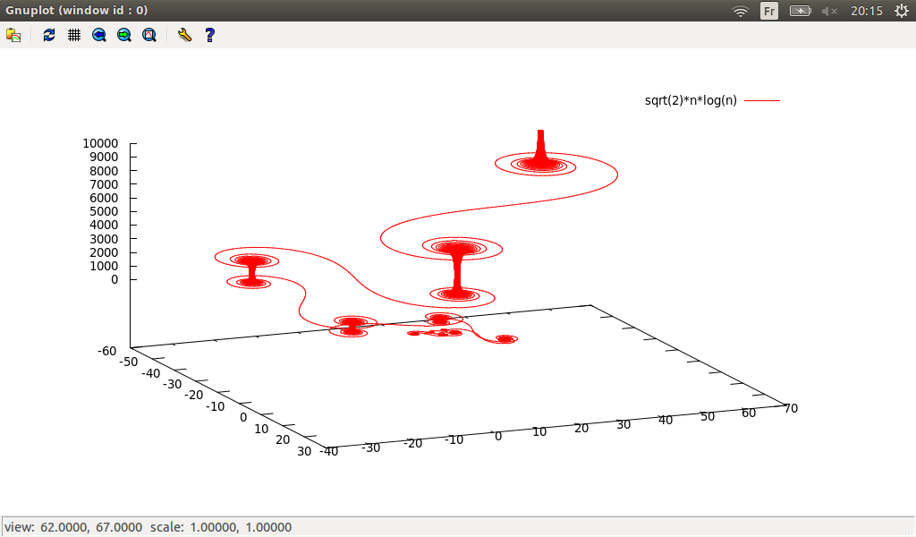
Next
un = n2 + 3n + 2 and
N = 10000:

Or
un = cos(n) and
N = 10000:
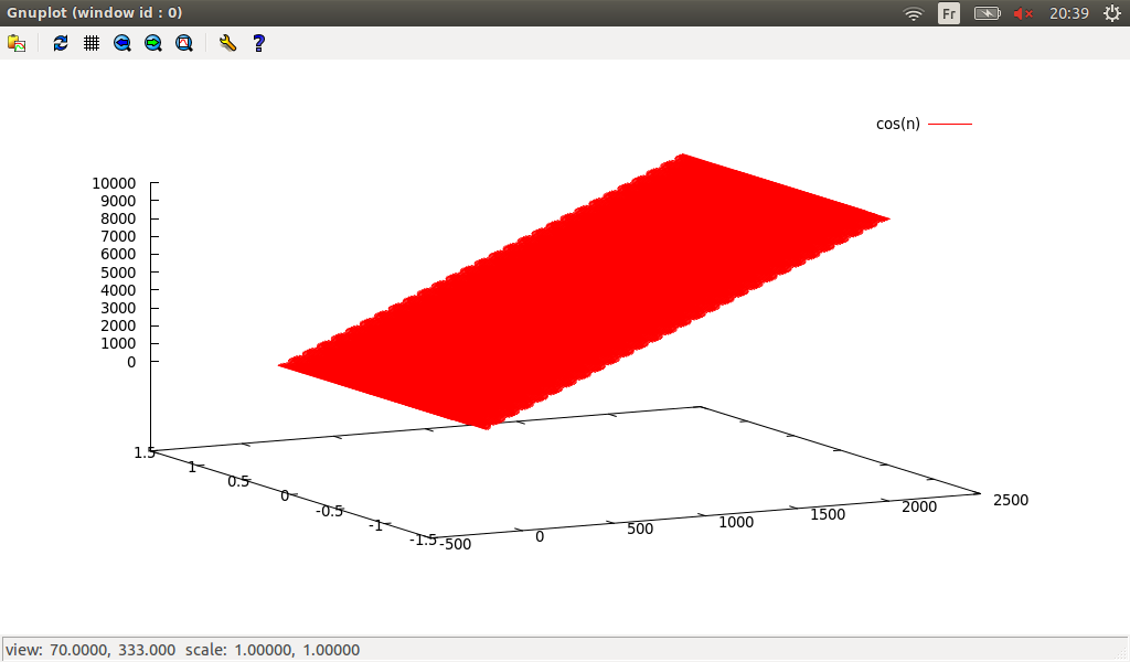
And finally
un = cos(√(2)nln(n)) and
N = 10000:
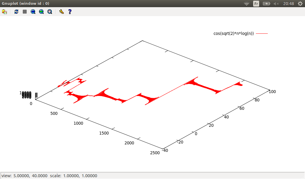
and changing point of view :
This time we are going to study graph theory through spectral theory. A graph is composed by a set of vertices and a set of edges. Here graphs are not oriented, hence adjacency matrix is symmetric and wee can use eigen function.
We compute :
-
order of graph↓ ↓ o: number of vertices,
-
↓↓size of graph s: number of edges,
-
density of graph↓↓ d = S⁄o2,
-
↓↓adjacency matrix A,
-
↓number of triangles = Tr(A3)⁄6
-
↓↓degree matrix D,
-
↓↓laplacian matrix L = D − A.
Using eigen, we can compute eigenvalue of laplacian matrix, the multiplicity of the eigenvalue 0 is the number of connected components
↓↓.
Example 1

So in smib :
Alp=(a,b,c,d)
Gra1=((a,b),(a,c),(c,d))
graphanalysis(Alp,Gra1)
And smib gives :
Order of graph = 4
Size of graph = 3
Density of graph = 3/16
Adjacency matrix of graph = ((0,1,1,0),(1,0,0,0),(1,0,0,1),(0,0,1,0))
Eigenvalues of adjacency matrix of graph = (1.61803,-1.61803,-0.618034,0.618034)
Number of triangles = 0
Laplacian matrix of graph = ((2,-1,-1,0),(-1,1,0,0),(-1,0,2,-1),(0,0,-1,1))
Eigenvalues of laplacian matrix of graph = (3.41421,8.71288e-17,2,0.585786)
Number of connected components of graph = 1
Example 2
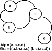
So in smib :
Alp=(a,b,c,d)
Gra2=((a,b),(a,c),(b,c),(c,d))
graphanalysis(Alp,Gra2)
And smib gives :
Order of graph = 4
Size of graph = 4
Density of graph = 1/4
Adjacency matrix of graph = ((0,1,1,0),(1,0,1,0),(1,1,0,1),(0,0,1,0))
Eigenvalues of adjacency matrix of graph = (2.17009,-1,-1.48119,0.311108)
Number of triangles = 1
Laplacian matrix of graph = ((2,-1,-1,0),(-1,2,-1,0),(-1,-1,3,-1),(0,0,-1,1))
Eigenvalues of laplacian matrix of graph = (-9.46217e-17,3,4,1)
Number of connected components of graph = 1
Example 3
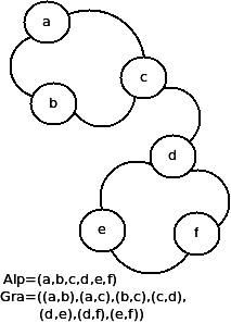
So in smib :
Alp=(a,b,c,d,e,f)
Gra3=((a,b),(a,c),(b,c),(c,d),(d,e),(d,f),(e,f))
graphanalysis(Alp,Gra3)
And smib gives :
Order of graph = 6
Size of graph = 7
Density of graph = 7/36
Adjacency matrix of graph =
((0,1,1,0,0,0),(1,0,1,0,0,0),(1,1,0,1,0,0),
(0,0,1,0,1,1),(0,0,0,1,0,1),(0,0,0,1,1,0))
Eigenvalues of adjacency matrix of graph = (2.41421,-1,-1.73205,1.73205,-0.414214,-1)
Number of triangles = 2
Laplacian matrix of graph =
((2,-1,-1,0,0,0),(-1,2,-1,0,0,0),(-1,-1,3,-1,0,0),
(0,0,-1,3,-1,-1),(0,0,0,-1,2,-1),(0,0,0,-1,-1,2))
Eigenvalues of laplacian matrix of graph = (-1.14369e-16,3,4.56155,3,0.438447,3)
Number of connected components of graph = 1
Example 4
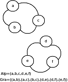
So in smib :
Alp=(a,b,c,d,e,f)
Gra4=((a,b),(a,c),(b,c),(d,e),(d,f),(e,f))
graphanalysis(Alp,Gra4)
And smib gives :
Order of graph = 6
Size of graph = 6
Density of graph = 1/6
Adjacency matrix of graph =
((0,1,1,0,0,0),(1,0,1,0,0,0),(1,1,0,0,0,0),
(0,0,0,0,1,1),(0,0,0,1,0,1),(0,0,0,1,1,0))
Eigenvalues of adjacency matrix of graph = (2,-1,-1,2,-1,-1)
Number of triangles = 2
Laplacian matrix of graph =
((2,-1,-1,0,0,0),(-1,2,-1,0,0,0),(-1,-1,2,0,0,0),
(0,0,0,2,-1,-1),(0,0,0,-1,2,-1),(0,0,0,-1,-1,2))
Eigenvalues of laplacian matrix of graph = (-9.11362e-17,3,3,-9.11362e-17,3,3)
Number of connected components of graph = 2
Example 5

So in smib :
Alp=(a,b,c,d,e)
Gra5=((a,b),(a,c),(a,d),(a,e),(b,c),(b,d),(b,e),(c,d),(c,e),(d,e))
graphanalysis(Alp,Gra5)
And smib gives :
Order of graph = 5
Size of graph = 10
Density of graph = 2/5
Adjacency matrix of graph =
((0,1,1,1,1),(1,0,1,1,1),(1,1,0,1,1),(1,1,1,0,1),(1,1,1,1,0))
Eigenvalues of adjacency matrix of graph = (4,-1,-1,-1,-1)
Number of triangles = 10
Laplacian matrix of graph =
((4,-1,-1,-1,-1),(-1,4,-1,-1,-1),(-1,-1,4,-1,-1),
(-1,-1,-1,4,-1),(-1,-1,-1,-1,4))
note: eigen did not converge
Eigenvalues of laplacian matrix of graph = (-3.55264e-16,5,5,5,5)
Number of connected components of graph = 1
N.B. :
-
On last example, we see that eigen function may give erratic result...
-
programs are not very difficult cf. init.cpp.
Let ℍ be the ring of quaternions, Mℍ = ⎧⎨⎩⎛⎜⎝
a + ib
c + id
− c + id
a − ib
⎞⎟⎠, a, b, c, d ∈ ℝ⎫⎬⎭, QI = ⎛⎜⎝
1
0
0
1
⎞⎟⎠, QA = ⎛⎜⎝
i
0
0
− i
⎞⎟⎠, QB = ⎛⎜⎝
0
1
− 1
0
⎞⎟⎠, QAB = QA.QB = ⎛⎜⎝
0
i
i
0
⎞⎟⎠ ((QI, QA, QB, QAB) forms a basis of Mℍ), h = (a1, b1, c1, d1) ∈ R4, l = (a2, b2, c2, d2) ∈ R4.
Morphisms between ℍ andMℍ :
QM:H⟶Mℍ, h⟼a1.QI + a2.QA + a3.QB + a4.QAB,
MQ:Mℍ⟶H, m = ⎛⎜⎝
a + ib
c + id
− c + id
a − ib
⎞⎟⎠⟼(a, b, c, d).
Operations on ℍ :
negation
↓ :
Qneg(h) = ( − a1, − a2, − a3, − a4),
conjugation
↓ :
Qconj(h) = (a1, − a2, − a3, − a4),
norm
↓ :
Qnorm(h) = √(∑j = 4j = 1a2i),
sum
↓ :
Qsum(h, l) = MQ(QM(h) + QM(l)),
product
↓ :
Qprod(h, l) = MQ(QM(h).QM(l)),
commutator
↓ :
Qcomm(h, l) = Qsum(Qprod(h, l), Qneg(Qprod(l, h))),
inverse
↓ :
Qinv(h) = Qconj(h)⁄Qnorm(h)2.
Some properties of operations :
-
Qsum(Qneg(H), H) = 0,
-
Qsum(Qneg(H), H) = 0,
-
Qprod(Qinv(H), H) = (1, 0, 0, 0),
-
Qprod(H, Qinv(H)) = (1, 0, 0, 0),
-
Qcomm(Qinv(H), H) = 0,
-
Qcomm(H, Qinv(H)) = 0,
-
Associativity↓ of the three operations.
So in smib :
And smib gives :
N.B. : All operations are associative, but it is not always like this; on the other side if we compare and and and , noncommutativity↓ of the multiplication and of the commutator is clear.
5.8.6 On ↓nonassociativity and Jacobi identity↓
-
in ℝ3 with flat metric :
ℝ3 is an eucliean vector space, we can define on this space the vector cross product↓↓. Let U = ⎛⎜⎜⎜⎝
ux
uy
uz
⎞⎟⎟⎟⎠ and V = ⎛⎜⎜⎜⎝
vx
vy
vz
⎞⎟⎟⎟⎠, the cross product is defined by U × V = ⎛⎜⎜⎜⎝
uyvz − uzvy
uzvx − uxvz
uxvy − uyvx
⎞⎟⎟⎟⎠ (in smib we use Levi-Civita symbol↓↓ crossP(U,V)=contr(contr(outer(LeviCivita(dim(U)),outer(U,V)),3,5),2,3)), we can show that the cross product is bilinear (i.e. (aU1 + bU2) × V = aU1 × V + bU2 × V and U × (aV1 + bV2) = aU × V1 + bU × V2). We want to verify :
-
U × (V × W) − (U × V) × W ≠ 0 : non-associativity
-
(U × V) × W + (V × W) × U + (W × U) × V = 0 : Jacobi identity
So in smib :
U1=(ux1,uy1,uz1)
U2=(ux2,uy2,uz2)
U3=(ux3,uy3,uz3)
test(crossP(crossP(U1,U2),U3)-crossP(U1,crossP(U2,U3))==0,
print("Associativity : Ok"),
print("Associativity : Ko"))
test(crossP(crossP(U1,U2),U3)+crossP(crossP(U2,U3),U1)+crossP(crossP(U3,U1),U2)==0,
print("Jacobi identity : Ok"),
print("Jacobi identity : Ko"))
And smib gives :
Associativity : Ko
Jacobi identity : Ok
-
In ℝ4 with non-flat metric↓↓ :
We consider the following symmetric metric↓↓ g = ⎛⎜⎜⎜⎜⎜⎝
f1
0
0
0
0
f2
0
0
0
0
f3
0
0
0
0
f4
⎞⎟⎟⎟⎟⎟⎠on , [u, v] = ∇vu − ∇uv is the commutator↓ which is also bilinear. We want to verify :
-
[U, [V, W]] − [[U, V], W] ≠ 0 : non-associativity
-
[[U, V], W] + [[V, W], U] + [[W, U], V] = 0 : Jacobi identity
So in smib :
X=(x0,x1,x2,x3)
W=(w0(X),w1(X),w2(X),w3(X))
V=(v0(X),v1(X),v2(X),v3(X))
U=(u0(X),u1(X),u2(X),u3(X))
symetricmetric= ((f1(X), 0, 0, 0),
(0, f2(X), 0, 0),
(0, 0, f3(X), 0),
(0, 0, 0, f4(X)))
riemann(symetricmetric,X)
test(Commutator(Commutator(U,V),W)-Commutator(U,Commutator(V,W))==0,
print("Associativity : Ok"),
print("Associativity : Ko"))
test(Commutator(Commutator(U,V),W)+Commutator(Commutator(V,W),U)+
Commutator(Commutator(W,U),V)==0,
print("Jacobi identity : Ok"),
print("Jacobi identity : Ko"))
And smib gives :
Associativity : Ko
Jacobi identity : Ok
The Gould number is defined by: (ln(6403203 + 744)⁄π)2, here we want to compute numerically this number, so in smib:
gould=(log(640320^3+744)/pi)^2
print("gould=",gould)
print("num(gould)=",num(gould))
So the computation gives:
gould= log(262537412640768744)^2/(pi^2)
num(gould)= 163
Here we see a ↓weakness of smib, Gould number is not an integer ...
5.8.8 ↓π computation (ten lessons for cooking π)
Here we want to test the following formulas:
-
↓↓Wallis formula: π = 2∏j = ∞j = 1(2j2)⁄(2j − 1)(2j + 1)
-
From Wallis formula: π = ∑j = ∞j = 02j + 1j!2⁄(2j + 1)!
-
Unknown man formula: π = 4(1 − ∑j = ∞j = 12⁄16j2 − 1)
-
↓Wang formula↓: π = 4(183arctan(1⁄239) + 32arctan(1⁄1023) − 68arctan(1⁄5832) +
12arctan(1⁄110443) − 12arctan(1⁄4841182) − 100arctan(1⁄6826318))
-
Using ζ ↓↓Riemann function: π = √(6∑j = ∞j = 11⁄j2)
-
Using sequence of prime numbers↓↓: π = √(6∏j ∈ P1⁄1 − 1⁄j2), where P is the set of prime numbers.
-
↓↓Ramanujan formula: 1⁄π = 2√(2)⁄9801∑j = ∞j = 1(4j)!(1103 + 26390j)⁄(j!43964j)
-
↓Chudnovsky formula↓: 1⁄π = 12∑j = ∞j = 0( − 1)j(6j)!13591409 + 545140134j⁄((3j)!j!3640320(3(j + 1 ⁄ 2)))
-
↓↓Bailey–Borwein–Plouffe formula: π = ∑j = ∞j = 016 − j[4⁄8j + 1 − 2⁄8j + 4 − 1⁄8j + 5 − 1⁄8j + 6]
-
↓↓Bellard formula: π = ∑j = ∞j = 0( − 1)j⁄210j[ − 25⁄4j + 1 − 1⁄4j + 3 + 28⁄10j + 1 − 26⁄10j + 3
− 22⁄10j + 5 − 22⁄10j + 7 + 1⁄10j + 9]
Those ten formulas can be implemented as:
prec=30
print("pi = ",num(pi))
print("Wallis: 2*product(ind,1,prec,(2*ind)^2/((2*ind-1)*(2*ind+1)))-pi=",
num(2*product(ind,1,prec,(2*ind)^2/((2*ind-1)*(2*ind+1)))-pi))
print("From Wallis: sum(ind,0,prec,2^(ind+1)*(ind!)^2/(2*ind+1)!)-pi=",
num(sum(ind,0,prec,2^(ind+1)*(ind!)^2/(2*ind+1)!)-pi))
print("4*(1-sum(ind,1,prec,2/(16*ind^2-1)))-pi = ",
num(4*(1-sum(ind,1,prec,2/(16*ind^2-1)))-pi))
print("Wang: 4*(183*arctan(1/239)+32*arctan(1/1023)-
68*arctan(1/5832)+12*arctan(1/110443)-
12*arctan(1/4841182)-100*arctan(1/6826318)-pi = ",
num(4*(183*arctan(1/239)+32*arctan(1/1023)-
68*arctan(1/5832)+12*arctan(1/110443)
12*arctan(1/4841182)-100*arctan(1/6826318))-pi))
print("With zeta function: sqrt(6*sum(ind,1,prec,1/ind^2))-pi = ",
num(sqrt(6*sum(ind,1,prec,1/ind^2))-pi))
print("With prime intergers: sqrt(6*product(ind,1,prec,test(isprime(ind)==1,
1/(1-ind^(-2)),1))-pi = ",
num(sqrt(6*product(ind,1,prec,test(isprime(ind)==1,1/(1-ind^(-2)),1)))-pi))
print("Ramanujan: 1/(2*sqrt(2)/9801*sum(ind,1,prec,
(4*ind)!*(1103+26390*ind)/(ind!^4*396^(4*ind)))-pi = ",
num(1/(2*sqrt(2)/9801*sum(ind,0,prec,(4*ind)!*
(1103+26390*ind)/(ind!^4*396^(4*ind))))-pi))
print("Chudnovsky: 1/(12*sum(ind,0,prec,(-1)^ind*(6*ind)!*(13591409+545140134*ind)/
((3*ind)!*(ind!)^3*640320^(3*(ind+1/2)))-pi = ",
num(1/(12*sum(ind,0,prec,(-1)^ind*(6*ind)!*(13591409+545140134*ind)/
((3*ind)!*(ind!)^3*640320^(3*(ind+1/2)))))-pi))
print("BBP: sum(ind,0,prec,16^(-ind)*(4/(8*ind+1)-2/(8*ind+4)-
1/(8*ind+5)-1/(8*ind+6)))-pi = ",
num(sum(ind,0,prec,16^(-ind)*(4/(8*ind+1)-2/(8*ind+4)-
1/(8*ind+5)-1/(8*ind+6)))-pi))
print("Bellard: sum(ind,0,prec,(-1)^ind/2^(10*ind)*(-2^5/(4*ind+1)-
1/(4*ind+3)+2^8/(10*ind+1)-2^6/(10*ind+3)-2^2/(10*ind+5)-
2^2/(10*ind+7)+1/(10*ind+9))/2^6-pi = ",
num(sum(ind,0,prec,(-1)^ind/2^(10*ind)*
(-2^5/(4*ind+1)-1/(4*ind+3)+2^8/(10*ind+1)-2^6/(10*ind+3)-
2^2/(10*ind+5)-2^2/(10*ind+7)+1/(10*ind+9)))/2^6-pi))
And smib gives :
5.8.9 Electromagnetic tensor↓↓
Let X = (t, x, y, z), f is a function depending on x, y and z, V = (Vx, Vy, Vz), each Vi depending on x, y and z too. We define the following operators :
-
grad(f) = ∇f = (∂xf, ∂yf, ∂zf),
-
div(V) = ∇.V = ∂xVx + ∂yVy + ∂zVz,
-
curl(V) = ∇ × V = ⎛⎜⎜⎜⎝
∂zVy − ∂yVz
∂zVx − ∂xVz
∂xVy − ∂yVx
⎞⎟⎟⎟⎠,
-
laplacian(f) = △f = ∂2xf + ∂2yf + ∂2zf.
So in smib :
X=(t,x,y,z)
grad(v) = d(v,(x,y,z))
div(v) = contract(d(v,(x,y,z)),1,2)
curl(f) = ( d(f[3],y) - d(f[2],z), d(f[1],z) - d(f[3],x), d(f[2],x) - d(f[1],y) )
laplacian(f) = d(d(f,x),x) + d(d(f,y),y) + d(d(f,z),z)
The vector potential is defined as: A = (Ax, Ay, Az), and electromagnetic four-potential as Aμ = (φ, Ax, Ay, Az); Minkowski metric is gμν = ⎛⎜⎜⎜⎜⎜⎝
1
0
0
0
0
− 1
0
0
0
0
− 1
0
0
0
0
− 1
⎞⎟⎟⎟⎟⎟⎠, using riemann function, we compute gμν, then Aμ = gμνAν. So in smib :
Au=(phi(),Ax(),Ay(),Az())
A=(Ax(),Ay(),Az())
Minkowski=((1,0,0,0),(0,-1,0,0),(0,0,-1,0),(0,0,0,-1))
gdd=Minkowski riemann(gdd,X)
Ad=contr(outer(gdd,Au),2,3)
Electromagnetic tensor is defined as Fμν = (dA)μν = ∂μAν − ∂νAμ, we can compute Fμν too, E = − ∂tA − ∇φ is electric field and B = ∇ × A is magnetic field, so in smib :
F1dd=d(Ad,X)-transpose(d(Ad,X),1,2)
F1uu=-contract(outer(guu,contract(outer(guu,F1dd),2,3)),2,4)
E=-d(A,t)-grad(phi())
B=curl(A)
Electromagnetic tensor yields the following properties :
-
Fμν = − Fνμ
-
FμνFμν = 2(B2 − E2)
-
det(Fμν) = (B.E)2
-
1⁄2ϵαβγδFαβFγδ = − 4(B.E)
So in smib :
F1uu+transpose(F1uu,1,2)==0
simplify(contract(contract(outer(F1dd,F1uu),1,3),1,2)-2*(B^2-E^2))==0
simplify(det(F1uu)-dot(B,E)^2)==0
1/2*contract(contract(contract(contract
(outer(LeviCivita(4),outer(F1uu,F1uu)),4,8),3,6),2,4),1,2)-4*dot(B,E)==0
Gauss law gives ρ = ∇.E, and Ampère law: J = ∇ × B − ∂tE, Jα = (ρ, Jx, Jy, Jz) is 4-current. We have :
-
Fαβ, γ + Fβγ, α + Fγα, β = 0
-
Fαβ, β = Jα
So in smib :
rho=div(E)
J=curl(B)-d(E,t)
Ju=(rho,J[1],J[2],J[3])
F1ddd = d(F1dd,X)
T1 = transpose(transpose(F1ddd,2,3),1,2)
T2 = transpose(transpose(F1ddd,1,2),2,3)
F1ddd + T1 + T2==0
contract(d(F1uu,X),2,3)-Ju==0
And smib gives (with some displays) only zeroes:
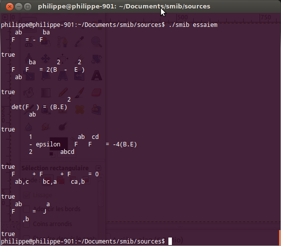
N.B. : we consider that ε0 = μ0 = c = 1 (it is just a question of units...)
6 Short bibliography
-
“Handbook of mathematical functions” (Abramovitz & Stegun) is a must read and a fabulous toolbox.
-
On number theory:
-
“1001 problèmes en théorie classique des nombres” (Koninck & Mercier),
-
“Thèmes d’arithmétique“ (Bordelles),
-
“Algebra” (Lang),
-
“A=B” (Marko Petkovsek, Herbert Wilf & Doron Zeilberger).
-
On analysis:
-
“Generalized Functions: Theory and Applications” (Kanwal),
-
“Eléments De Distributions Et D’équations Aux Dérivées Partielles” & “Problèmes de distributions avec solutions détaillées” (Zuily),
-
“Fourier transform” (Sneddon),
-
“Eléments De La Théorie Des Fonctions Et De L’analyse Fonctionnelle” (Kolmogorov & Fomine),
-
“A Treatise On Differential Equations” (Forsyth),
-
“Intégration et analyse de Fourier. Probabilités et analyse gaussienne” (Malliavin & Airault),
-
“Intégration Et Probalités, Analyse De Fourier - Exercices Corrigés” (Letac),
-
“Analyse continue par ondelettes” (Torrésani & Meyer),
-
“Distribution theory and transform analysis” (Zemanian),
-
“Calcul différentiel complexe” (Leborgne),
-
“The Fractional Calculus” (Oldham & Spanier),
-
“Methods of Numerical Integration” (Rabinowitz & Davis),
-
“Symbolic integration I” (Bronstein),
-
“Calcul formel” (Davenport, Siret & Tournier).
-
On vector and tensor calculus, differential geometry:
-
“Schaum’s Outline of Vector Analysis” (Spiegel),
-
“Schaum’s Outline of Tensor Calculus” (Kay),
-
“Vector analysis” (Brand),
-
“Calcul tensoriel en physique” (Hladik),
-
“Calcul différentiel et géométrie” (Leborgne),
-
“Géométrie différentielle: variétés, courbes et surfaces” (Berger & Gostiaux).
-
On probability & statistic:
-
“Probabilites Et Statistique - Cours Et Problèmes” (Spiegel),
-
“Les Probabilités Et La Statistique De A à Z” (Dress),
-
“Introduction au calcul stochastique appliqué à la finance” (Lamberton & Lapeyre),
-
“Stochastic Simulation: Algorithms and Analysis” (Asmussen & Glynn).
-
“Méthodes de Monte-Carlo et processus stochastiques : du linéaire au non-linéaire” (Gobet)
-
“Introduction to stochastic analysis and Malliavin calculus” (Da Prato)
-
Miscellanous:
-
“Atlas des Mathématiques” (Reinhardt & Soeder),
-
“Quantique” (Elbaz),
-
“Leçons sur la gravitation” (Feynman),
-
“Dictionnaire des mathématiques” (Bouvier, George & Le Lionnais).
7 Glossary
Nomenclature
↑abs absolute value modulus
↑antider antiderivative of a function
↑argch hyperbolic cosinus argument
↑arggd Guderman function argument
↑argsh hyperbolic sinus argument
↑argth hyperbolic tangent argument
↑bernoulliN Bernoulli number
↑besseli besselj besselk Bessel functions
↑binomial binomial coefficient
↑ceiling integer part (smaller)
↑charpoly characteristic polynomial
↑convolution convolution product of two expressions
↑coth hyperbolic cotangent
↑csch hyperbolic cosecant
↑cyclotomic cyclotomic polynomial
↑d derivative (or partial derivative) of an expression
↑defint definite integral
↑deg degree of a polynomial
↑derangement derangement number
↑dilatation abscissa dilatation
↑dim vector or matrix dimension
↑dirichletproduct Dirichlet convolution product
↑discpoly discriminant of a polynomial
↑divpoly euclidian division
↑dot product of a matrix by a vector
↑egcdpoly extended greater common divisor of polynomials
↑eigen eigenvalues and eigenvectors of a symmetric matrix
↑erf erfc error functions
↑eulerN1k Euler number of first kind
↑eulerN2k Euler number of second kind
↑eulerphi Euler totient function
↑expand expansion of expression
↑factor integer factorization
↑fibonacciN Fibonacci number
↑float floating point conversion
↑floor integer part (greater)
↑fourier Fourier transform of an expression
↑fracdec decomposition of a rational fraction
↑frobeniusnorm Frobenius norm
↑Gamma Gamma Euler function
↑gcd great common divisor
↑gcdpoly greater common divisor of polynomials
↑genocchiN Genocchi number
↑gnuplot2D convert a 2D sample into datas usable by gnuplot or qgfe
↑gnuplot3D convert 3D sample into data usable by gnuplot (or qgfe)
↑hermite Hermite polynomial
↑incrdivpoly increasing power division
↑integerkernel kernel of integer
↑integral integration of an expression
↑invfourier inverse Fourier transform of an expression
↑isprime is prime integer
↑jacobisymbol Jacobi symbol
↑laguerre Laguerre polynomial
↑lcm least common divisor
↑legendre Legendre polynomial
↑legendresymbol Legendre symbol
↑limit limit of a function
↑liouvillefunction Liouville function
↑mangoldt van Mangoldt function
↑mersenneN Mersenne number
↑mertens Mertens function
↑modulation modulation (product of an expression by a complex exponential)
↑nil ex nihilo, quod libet.
↑noisevector stochastic vector
↑normnoisevector(n,s) normal aleatory number vector.
↑normrand(x) random number (normal distribution)
↑nroot roots of a polynomial (numerical method)
↑num(z) floating point conversion of complex
↑numint numerical integration (using Simpson or Gauss method depending on simpsonint).
↑odesolve first and second order linear unhomogeneous ordinary differential equation solver
↑Omega total number of prime factors
↑permutation permutation number
↑primedecomp prime integer decomposition
↑productoverdivisor product over divisors of an integer
↑productoverprime product over prime divisors of an integer
↑prog program declaration
↑random pseudo-aleatory rational (uniform distribution)
↑rationalize reduction to same denominator
↑resultant resultant of polynomials
↑Sabs absolute value (modulus) of a sample
↑sample sample a function
↑Sarg argument of a complex sample
↑Sd derivative of a sample
↑Sdecomp extraction of a column of a sample
↑Sdefint definite integral of a sample
↑Sdelete delete ith column of a sample.
↑Sdiff difference between samples
↑Sdiscconvolution convolution product of two samples
↑Sdiscfourier Fourier transform of a sample
↑Sdiscinvfourier inverse Fourier transform of sample
↑Sfracd fractional derivative of a sample to a non integer order
↑sigma sum of divisors at order r
↑Simag imaginary part of a complex sample
↑simplify simplification of expression
↑simpson numerical integration (using Simpson method)
↑Sint integral of a sample
↑Sproduct product of two samples
↑squarefreepoly squarefree factorization of polynomial
↑Sreal real part of a complex sample
↑Srecomp fusion of two columns forming a sample
↑Sscalarproduct product of a scalar and a sample
↑stirlingN1k Stirling number of first kind
↑stirlingN2k Stirling number of second kind
↑sumoverdivisor sum over divisors of an integer
↑sumoverprime sum over prime divisors of an integer
↑taylor Taylor partial sum
↑tchebychevT T Tchebychev polynomial
↑tchebychevU U Tchebychev polynomial
↑translation abscissa translation
Index
2D curves: ↑
2D plotting: ↑
3D curves: ↑
3D dynamic system: ↑
3D plotting: ↑
Airy functions: ↑
Archimedes constant: ↑
Bailey-Borwein-Plouffe formula: ↑
Bell number: ↑
Bellard formula: ↑
Bernoulli distribution: ↑
Bernoulli number: ↑, ↑
Bessel function of first kind: ↑
Bessel function of second kind: ↑
Bessel functions: ↑
Bessel modified function of first kind: ↑
Bessel modified function of second kind: ↑
Beta binomial distribution: ↑
Beta distribution: ↑
Beta function: ↑
Beta prime distribution: ↑
Bezout identity: ↑
Black-Scholes-Merton process: ↑, ↑
Bloch sphere: ↑
Bombieri conjecture: ↑
Bonhoeffer Van der Pool oscillator: ↑
Bonnet theorem: ↑
Borel-Tanner distribution: ↑
Bose-Einstein distribution: ↑
Box-Muller method: ↑
Box-Muller transform: ↑
Catalan number: ↑
Cauchy distribution: ↑
Christoffel symbol: ↑, ↑
Chudnovsky formula: ↑
Cox-Ingersoll-Ross process: ↑
De Morgan’s law: ↑
Dirichlet convolution product: ↑
Dirichlet product: ↑
Duffing-Van der Pool oscillator: ↑
Einstein tensor: ↑
Erlang distribution: ↑
Euler constant: ↑
Euler method: ↑
Euler numbers of first and second kind: ↑
Euler totient function: ↑
Euler-Maruyama method: ↑, ↑
F distribution: ↑
Fermat number: ↑
Fermi-Dirac distribution: ↑, ↑
Feynman-Kac formula: ↑
Fibonacci number: ↑, ↑
Fourier tranform of sample: ↑
Fourier transform: ↑
Fourier transform, continous: ↑
Fourier transform, discrete: ↑
Frobenius norm: ↑
Gamma distribution: ↑
Gamma function: ↑
Gauss equations: ↑
Gauss scheme: ↑, ↑, ↑, ↑, ↑, ↑
Gauss theorem: ↑
Gauss theory of surface: ↑
Gauss-Newton method: ↑
Gauss-Ostrogradski theorem: ↑
Genocchi number: ↑, ↑
Gibrat distribution: ↑
Gosper algorithm: ↑
Gould number: ↑
Green function: ↑
Green theorem: ↑
Grünwald definition: ↑
Grünwald definition, modified version of the: ↑
Guderman function: ↑
Hankel function of first kind: ↑
Hankel function of second kind: ↑
Hermite function: ↑
Hermite polynomial: ↑, ↑
Hermitian operators: ↑
Hilbert space: ↑
Ito’s lemma: ↑
Jacobi identity: ↑
Jacobi symbol: ↑, ↑
Lagrange interpolation problem: ↑
Laguerre polynomial: ↑, ↑
Laplace distribution: ↑
Laplace operator: ↑, ↑
Legendre polynomial: ↑, ↑
Legendre symbol: ↑
Levi-Civita symbol: ↑
Liouville function: ↑
Lorenz system: ↑, ↑
Lotka-Volterra equation: ↑
Mainardi-Codazzi equations: ↑
Maxwell distribution: ↑
Mersenne number: ↑, ↑
Mertens function: ↑, ↑
Milstein method: ↑, ↑
Möbius function: ↑
NAND: ↑
Newton basis polynomials: ↑
Newton method: ↑
Nil: ↑
Ornstein-Uhlenbeck process: ↑, ↑
Pareto distribution: ↑
Poisson distribution: ↑
Poisson law: ↑
Ramanujan formula: ↑
Rayleigh distribution: ↑
Redheffer matrix: ↑
Ricci curvature: ↑, ↑
Ricci scalar: ↑
Ricci tensor: ↑, ↑
Riemann function: ↑
Riemann method: ↑
Riemann scheme: ↑
Riemann tensor: ↑, ↑
Riemannian geometry: ↑
Risch algorithm: ↑
Runge-Kutta method: ↑
Rössler system: ↑, ↑
Schrodinger equation: ↑
Schwarzschild metric: ↑
Simpson method: ↑
Simpson numerical scheme: ↑
Simpson scheme: ↑, ↑, ↑, ↑, ↑
Sol: ↑
Solovay-Strassen test: ↑
Stirling numbers of first and second kind: ↑
Stokes theorem: ↑
Stratonovich calculus: ↑
Student-t distribution: ↑
Student-z distribution: ↑
Syracuse problem: ↑
Taylor partial sum: ↑
Tchebychev polynomial: ↑
Vasicek process: ↑
Wallis formula: ↑
Wang formula: ↑
Weibull distribution: ↑
Weingarten operator: ↑
Weyl sum: ↑
Wilson formula: ↑
Yun algorithm: ↑
Yun square free factorization: ↑
absolute value: ↑
absolute value of a sample: ↑
acceleration vector: ↑
adjacency matrix: ↑
adjoint: ↑
algorithm, Gosper: ↑
algorithm, Yun: ↑
algorithm, euclidean: ↑
algorithm, extended euclidean: ↑
annihilation: ↑
antider: ↑, ↑
antiderivative: ↑, ↑
antidifference: ↑
antilogy: ↑
area integral: ↑
argument: ↑
argument of a sample: ↑
arithmetic equations: ↑
arithmetic function: ↑
associativity: ↑
binomial coefficient: ↑
binomial distribution: ↑
binormal vector: ↑
boolean indicators: ↑
bra: ↑
brownian motion: ↑, ↑
central limit theorem: ↑
characteristic polynomial: ↑
chi distribution: ↑
chi squared distribution: ↑
chinese remainder theorem: ↑
circle: ↑
coefficient, connection: ↑
coefficient, correlation: ↑
coin-tossing: ↑
commutator: ↑, ↑, ↑
compilation: ↑
complex analysis: ↑
complex numbers: ↑
complex path integral: ↑, ↑
condition: ↑
conjugate: ↑
conjunction: ↑
connected components, number of: ↑
connection coefficient: ↑, ↑
constant, Archimedes: ↑
constant, Euler: ↑
continous Fourier transform: ↑
contraposition: ↑
convolution product: ↑, ↑
convolution product of two samples: ↑
coordinate, orthogonal: ↑
correlation coefficient: ↑
covariant derivative: ↑, ↑
covariant derivative of tensor: ↑
creation: ↑
curl: ↑
curl of a vector field: ↑
curvature: ↑, ↑
curvature, Ricci: ↑, ↑
curvature, gaussian: ↑
curvature, mean: ↑
curvature, principal: ↑
curvedness: ↑
curvilinear integral: ↑
cyclotomic polynomial: ↑
cylinder: ↑
decomposition of a rational function: ↑
decomposition of rational function: ↑
definite integral of a sample: ↑
degree matrix: ↑
degree of a polynomial: ↑
denominator: ↑
density of graph: ↑
derangement: ↑
derivation of non-integer order: ↑
derivative: ↑
derivative of a sample: ↑
derivative, covariant: ↑, ↑
derivative, directed covariant: ↑
determinant: ↑, ↑
deterministic test: ↑
difference between two samples: ↑
differential equation: ↑, ↑
differential equation, higher order ordinary: ↑
differential equation, stochastic: ↑
differential equations, system of: ↑
differential geometry: ↑
differential operator: ↑
differintegration: ↑
dilatation: ↑
dimension of a vector: ↑
directed covariant derivative: ↑
discrete Fourier transform: ↑
discrete moment: ↑
discriminant: ↑
disjunction: ↑
disjunction, exclusive: ↑
distribution: ↑
distribution Fermi-Dirac: ↑
distribution function: ↑
distribution, Bernoulli: ↑
distribution, Beta: ↑
distribution, Beta binomial: ↑
distribution, Beta prime: ↑
distribution, Borel-Tanner: ↑
distribution, Bose-Einstein: ↑
distribution, Cauchy: ↑
distribution, Erlang: ↑
distribution, F: ↑
distribution, Fermi-Dirac: ↑
distribution, Gamma: ↑
distribution, Gibrat: ↑
distribution, Laplace: ↑
distribution, Maxwell: ↑
distribution, Pareto: ↑
distribution, Poisson: ↑
distribution, Rayleigh: ↑
distribution, Student-t: ↑
distribution, Student-z: ↑
distribution, Weibull: ↑
distribution, binomial: ↑
distribution, chi: ↑
distribution, chi squared: ↑
distribution, exponential: ↑, ↑
distribution, extreme value: ↑
distribution, geometric: ↑
distribution, half normal: ↑
distribution, inverse gaussian: ↑
distribution, log series: ↑
distribution, log-normal: ↑
distribution, logarithmic: ↑
distribution, logistic: ↑
distribution, multinomial: ↑
distribution, negative binomial: ↑
distribution, normal: ↑, ↑
distribution, uniform: ↑, ↑
distribution, von Mises: ↑
distribution, z: ↑
distributivity: ↑
divergence: ↑, ↑
divergence of a vector field: ↑
divide differences: ↑
division, euclidean: ↑
divisor, great common: ↑
divisors, number of: ↑, ↑
divisors, product over: ↑
divisors, sum over: ↑
eigenstates: ↑
eigenvalue of symmetric matrix: ↑
eigenvalues: ↑
eigenvector of symmetric matrix: ↑
electromagnetic tensor: ↑
electron spin: ↑
equality: ↑, ↑
equation, Gauss: ↑
equation, Lotka-Volterra: ↑
equation, Mainardi-Codazzi: ↑
equation, Schrodinger: ↑
equation, arithmetic: ↑
equation, heat: ↑, ↑
equation, higher order ordinary differential: ↑
equation, ordinary differential: ↑, ↑
equation, partial differential: ↑
equation, stochastic differential: ↑
equations, system of differential: ↑
error functions: ↑
euclidean algorithm: ↑
euclidean division: ↑
euclidian division: ↑
even: ↑
exclusive disjunction: ↑
expansion of expression: ↑
exponential: ↑
exponential distribution: ↑, ↑
exponential function: ↑
extended euclidean algorithm: ↑
extented greater common divisor: ↑
extreme value distribution: ↑
factorial: ↑
factorization: ↑
factorization in prime factors: ↑
factorization, square-free: ↑
field of rational functions: ↑
first form: ↑
first kind, Bessel function of: ↑
first kind, Bessel modified function of: ↑
first kind, Euler numbers of: ↑
first kind, Hankel function of: ↑
first kind, Stirling numbers of: ↑
floating point conversion: ↑
form, first: ↑
form, second: ↑
formula, Bailey-Borwein-Plouffe: ↑
formula, Bellard: ↑
formula, Chudnovsky: ↑
formula, Feynman-Kac: ↑
formula, Ramanujan: ↑
formula, Wallis: ↑
formula, Wang: ↑
formula, Wilson: ↑
fractional calculus: ↑
fractional derivative of a sample: ↑
function: ↑
function, Airy: ↑
function, Bessel: ↑, ↑
function, Bessel modified: ↑
function, Beta: ↑
function, Euler totient: ↑
function, Gamma: ↑
function, Green: ↑
function, Guderman: ↑
function, Hankel: ↑
function, Hermite: ↑
function, Liouville: ↑
function, Mertens: ↑, ↑
function, Möbius: ↑
function, Riemann: ↑
function, arithmetic: ↑
function, distribution: ↑
function, error: ↑
function, exponential: ↑
function, greater integer: ↑
function, hyperbolic trigonometric: ↑, ↑
function, hypergeometric: ↑
function, inverse hyperbolic trigonometric: ↑, ↑
function, inverse trigonometric: ↑, ↑
function, logarithmic: ↑, ↑
function, rational: ↑
function, smaller integer: ↑
function, trigonometric: ↑, ↑
function, von Mangoldt: ↑
functions acting on integers: ↑
gaussian curvature: ↑
gcd: ↑
geometric distribution: ↑
gradient: ↑
gradient of a scalar field: ↑
graph: ↑
graph, density of: ↑
graph, order of: ↑
graph, size of: ↑
great common divisor: ↑
greater common divisor: ↑, ↑
greater integer function: ↑
half normal distribution: ↑
hamiltonian: ↑
harmonic mean of divisors: ↑
heat equation: ↑, ↑
helix: ↑
higher order ordinary differential equation: ↑
histogram: ↑, ↑
hyperbolic trigonometric function: ↑
hyperbolic trigonometric functions: ↑
hypergeometric distribution: ↑, ↑
hypergeometric function: ↑
identity, Bezout: ↑
imaginary part: ↑
imaginary part of a sample: ↑
implication: ↑
impulsion: ↑
increasing power division: ↑
index of a path: ↑
index, shape: ↑
inequality: ↑
infinity: ↑
inner product: ↑
integer: ↑
integer part: ↑
integer, kernel of: ↑
integral: ↑, ↑, ↑
integral by parts: ↑
integral of a sample: ↑
integral on compact: ↑
integral on semi-finite interval: ↑
integral, area: ↑
integral, complex path: ↑, ↑
integral, curvilinear: ↑
integral, miscellanous: ↑
integral, oscillatory: ↑
integral, vectorial: ↑
integration by part: ↑
interactive mode: ↑
interpolation: ↑
interpolation, polynomial: ↑
inverse: ↑
inverse gaussian distribution: ↑
inverse hyperbolic trigonometric function: ↑
inverse hyperbolic trigonometric functions: ↑
inverse trigonometric function: ↑
inverse trigonometric functions: ↑
inversion method: ↑
inversion problem: ↑
inversion, modular: ↑
isinteger: ↑
isprime: ↑
kernel of integer: ↑
kernel of the operator: ↑
ket: ↑
kurtosis: ↑, ↑, ↑, ↑
laplacian: ↑, ↑
laplacian matrix: ↑
laplacian of a scalar field: ↑
laplacian of a vector field: ↑
law of large numbers: ↑
least common multiple: ↑
limit: ↑
linear least squares fitting: ↑
log series distribution: ↑
log-normal distribution: ↑
logarithmic distribution: ↑
logarithmic function: ↑, ↑
logic conjonction: ↑
logic disjonction: ↑
logic negation: ↑
logical NAND: ↑
logical conjunction: ↑
logical disjunction: ↑
logical equality: ↑
logical exclusive disjunction: ↑
logical implication: ↑
logical negation: ↑
logical operator: ↑
logistic distribution: ↑
loop: ↑
lowering indices: ↑
matrices: ↑
matrix, Redheffer: ↑
matrix, adjacency: ↑
matrix, degree: ↑
matrix, laplacian: ↑
mean: ↑
mean curvature: ↑
median: ↑, ↑
median of a sample: ↑
median, quantile of a: ↑
method, Box-Muller: ↑
method, Euler: ↑
method, Euler-Maruyama: ↑, ↑
method, Gauss-Newton: ↑
method, Milstein: ↑, ↑
method, Newton: ↑
method, Riemann: ↑
method, Runge-Kutta: ↑
method, Simpson: ↑
metric: ↑, ↑
metric, Nil: ↑
metric, Schwarzschild: ↑
metric, Sol: ↑
metric, non-flat: ↑
metric, statical-spherical: ↑
metric, symmetric: ↑
miscellanous integrals: ↑
mode, interactive: ↑
mode, script: ↑
model, predator-prey: ↑
modified version of the Grünwald definition: ↑
modular inversion: ↑
modulation: ↑
modus barbara: ↑
modus ponens: ↑
modus tollens: ↑
moment: ↑
multinomial distribution: ↑
multiple, least common: ↑
negation: ↑
negative binomial distribution: ↑
nil: ↑, ↑
non-flat metric: ↑
non-integer order, derivation: ↑
non-linear least squares mean: ↑
nonassociativity: ↑
noncommutativity: ↑
norm of sample: ↑
normal distribution: ↑, ↑, ↑
normal vector: ↑, ↑, ↑
nth component: ↑
number of connected components: ↑
number of distinct prime factors: ↑
number of divisors: ↑, ↑
number of singularities: ↑
number of triangles: ↑
number, Bell: ↑
number, Bernoulli: ↑, ↑
number, Catalan: ↑
number, Euler: ↑
number, Fermat: ↑
number, Fibonacci: ↑, ↑
number, Genocchi: ↑, ↑
number, Gould: ↑
number, Mersenne: ↑, ↑
number, Stirling: ↑
numbers, prime: ↑
numerator: ↑
numerical analysis: ↑
numerical integration scheme: ↑
numerical scheme of integration: ↑
observable: ↑
odd: ↑
operator: ↑, ↑
operator acting on function: ↑
operator, Laplace: ↑
operator, Weingarten: ↑
operator, differential: ↑
operator, kernel of the: ↑
operator, logical: ↑
operator, pseudo-differential: ↑
operator, symbol of: ↑
order of graph: ↑
ordinary differential equation: ↑
ordinary differential equation solver: ↑
orthogonal coordinate: ↑
orthogonal polynomial: ↑, ↑
oscillator, Bonhoeffer Van der Pool: ↑
oscillator, Duffing-Van der Pool: ↑
oscillatory integral: ↑
oscillatory integral on semi-finite interval: ↑
outer product: ↑
partial differential equation: ↑
partial product: ↑
partial sum: ↑
partial sum, Taylor: ↑
path in the complex plane: ↑
path, complex integral: ↑
path, index of a: ↑
perfect number: ↑
permutation: ↑
photon: ↑
pi computation: ↑
planar curves: ↑
plotting: ↑
polar coordinates: ↑
polynomial: ↑, ↑
polynomial equation: ↑
polynomial interpolation: ↑
polynomial, Hermite: ↑, ↑
polynomial, Laguerre: ↑, ↑
polynomial, Legendre: ↑, ↑
polynomial, Tchebychev: ↑
polynomial, characteristic: ↑
polynomial, cyclotomic: ↑
polynomial, orthogonal: ↑, ↑
polynomial, roots of a: ↑
polynomials: ↑
position: ↑
position vector: ↑
predator-prey model: ↑
primality test: ↑
primality tests: ↑
prime counting: ↑
prime number theorem: ↑
prime numbers: ↑
primes, product over: ↑
primes, sum over: ↑
principal curvature: ↑
probabilistic test: ↑
probalility: ↑
process, Black-Scholes-Merton: ↑, ↑
process, Cox-Ingersoll-Ross: ↑
process, Ornstein-Uhlenbeck: ↑, ↑
process, Vasicek: ↑
product of a scalar and a sample: ↑
product of matrix by vector: ↑
product of two samples: ↑
product over divisors: ↑, ↑
product over prime divisors: ↑
product over primes: ↑
product, Dirichlet: ↑
product, Dirichlet convolution: ↑
product, convolution: ↑
product, partial: ↑
product, vector cross: ↑
program: ↑
programming language: ↑
projection: ↑
projector: ↑
proposition: ↑
propositional logic: ↑
pseudo-aleatory rational: ↑
pseudo-differential operator: ↑
quadratic variation: ↑
quanta number: ↑
quantile: ↑, ↑, ↑, ↑
quantile of a sample: ↑
quantum mechanic: ↑
quaternion: ↑
quaternion commutator: ↑
quaternion conjugation: ↑
quaternion inverse: ↑
quaternion negation: ↑
quaternion norm: ↑
quaternion product: ↑
quaternion sum: ↑
raising indices: ↑
random number: ↑
rational function: ↑, ↑
rational function, decomposition of: ↑
rational function, decomposition of a: ↑
rationnal numbers: ↑
real numbers: ↑
real part: ↑
real part of a sample: ↑
recursive loop: ↑
reduction to same denominator: ↑
resultant: ↑
roots of a polynomial: ↑
sample: ↑, ↑, ↑
sample filtering: ↑
sample truncation: ↑
sample, Fourier tranform of: ↑
sample, absolute value of a: ↑
sample, argument of a: ↑
sample, definite integral of a: ↑
sample, derivative of a: ↑
sample, fractional derivative of a: ↑
sample, imaginary part of a: ↑
sample, integral of a: ↑
sample, norm of: ↑
sample, product of a scalar and a: ↑
sample, quantile of a: ↑
sample, real part of a: ↑
samples, difference between two: ↑
samples, product of two: ↑
samples, sum of two: ↑
scalar field, gradient of a: ↑
scalar field, laplacian of a: ↑
scheme, Gauss: ↑, ↑, ↑
scheme, Simpson: ↑
script mode: ↑
second form: ↑
second kind, Bessel function of: ↑
second kind, Bessel modified function of: ↑
second kind, Euler numbers of: ↑
second kind, Hankel function of: ↑
second kind, Stirling numbers of: ↑
shape index: ↑
simplification of expression: ↑
singularities, number of: ↑
size of graph: ↑
skewness: ↑, ↑, ↑, ↑
smaller integer function: ↑
speed vector: ↑
sphere: ↑
spherical coordinates: ↑
square free factorization: ↑
square-free factorization: ↑
statical-spherical metric: ↑
statistic: ↑
stochastic differential equation: ↑
stochastic vector: ↑
sum: ↑
sum of divisors at order r: ↑
sum of two samples: ↑
sum over divisors: ↑, ↑
sum over primes: ↑
sum, Weyl: ↑
sum, partial: ↑
sum, partial Taylor: ↑
support: ↑
symbol of operator: ↑
symbol, Christoffel: ↑, ↑
symbol, Jacobi: ↑, ↑
symbol, Legendre: ↑
symbol, Levi-Civita: ↑
symmetric metric: ↑
system of differential equations: ↑
system, 3D dynamic: ↑
system, Lorenz: ↑
system, Rössler: ↑
tangent vector: ↑, ↑
tautology: ↑
temporary program: ↑, ↑
tensor: ↑
tensor product: ↑
tensor, Einstein: ↑
tensor, Ricci: ↑, ↑
tensor, Riemann: ↑, ↑
tensor, covariant derivative of: ↑
tensor, electromagnetic: ↑
theorem, Bonnet: ↑
theorem, Gauss: ↑
theorem, Gauss-Ostrogradski: ↑
theorem, Green: ↑
theorem, Stokes: ↑
theorem, central limit: ↑
theorem, chinese remainder: ↑
torsion: ↑
torus: ↑
total number of prime factors: ↑
trace: ↑
transform, Box-Muller: ↑
translation: ↑
transposition: ↑
trigonometric function: ↑, ↑
trigonometric functions: ↑
truth table: ↑
unidimensional integral calculus: ↑
uniform distribution: ↑, ↑, ↑
unity exponential: ↑
variance: ↑, ↑
vector cross product: ↑
vector field, curl of a: ↑
vector field, divergence of a: ↑
vector field, laplacian of a: ↑
vector, acceleration: ↑
vector, binormal: ↑
vector, normal: ↑, ↑, ↑
vector, position: ↑
vector, speed: ↑
vector, tangent: ↑, ↑
vectorial calculus: ↑
vectorial integral: ↑
vectors: ↑
von Mangoldt function: ↑
von Mises distribution: ↑
wavelet: ↑, ↑
weakness: ↑, ↑, ↑, ↑, ↑
wronskian: ↑
z distribution: ↑